Training Systems

If a model can generate text on a single accelerator card, does that mean it can also be trained on that card?

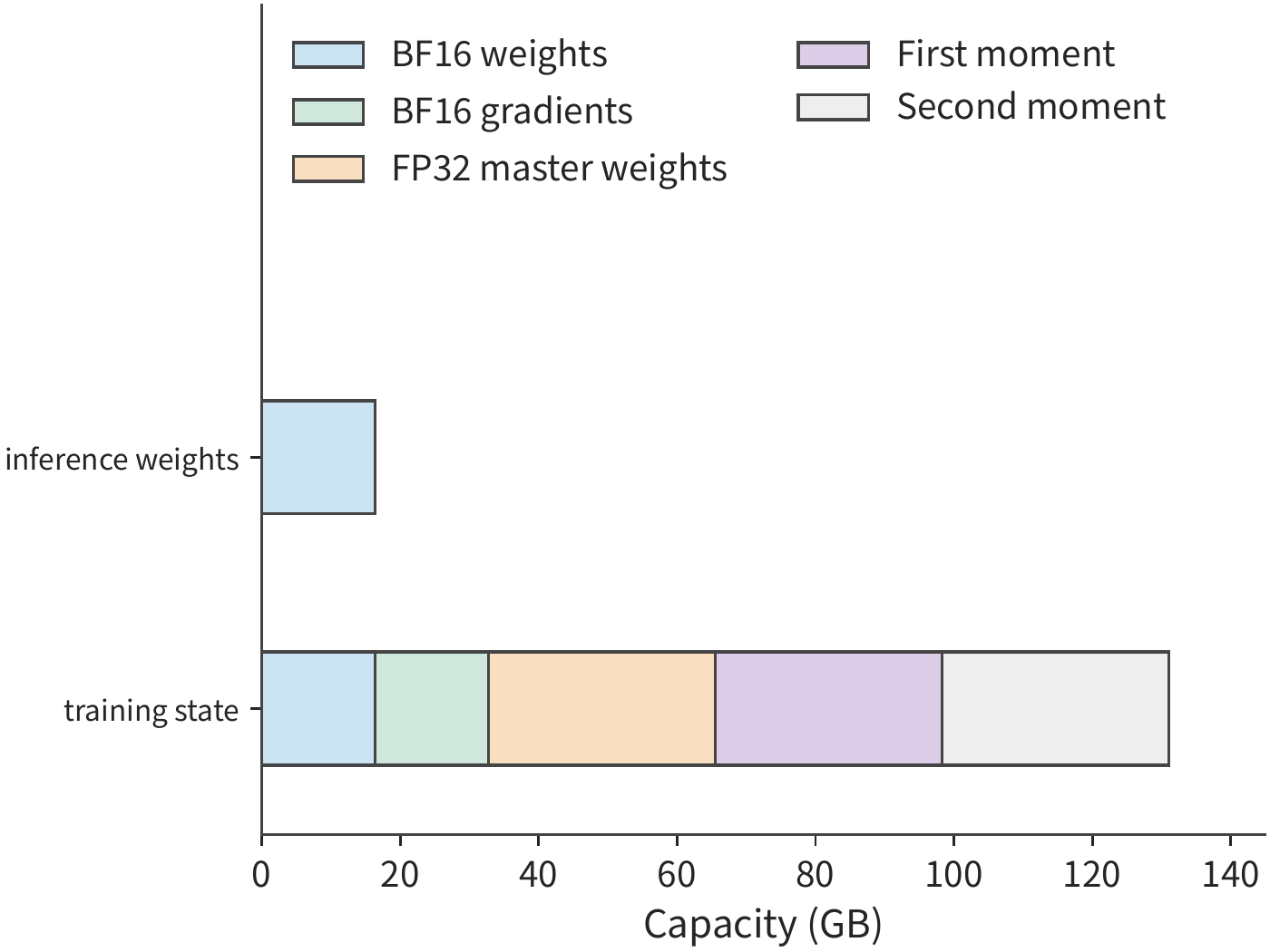
Full-parameter training updates every trainable weight in the model. Qwen3-8B's BF16 weights total about 16.4 GB, but when full-parameter training uses mixed-precision Adam, the system must also keep gradients, FP32 master weights, and the gradient history that Adam retains across steps, alongside the model weights, totaling about 131 GB. This training state occupies roughly eight times the space of the BF16 weights.

Backpropagation must read the activations retained from the forward pass; buffers for parameter gathering and format conversion are also needed during execution. Designing a training system starts with determining where these tensors and buffers reside, and how long they must be retained.

Splitting the training state across more cards can relieve per-card memory pressure, but computation then often waits on data arriving from other cards. Moving state to host memory frees up GPU memory but adds transfer overhead between host and GPU. When training runs for weeks, waiting for input, saving checkpoints, and repeating computation after failures all affect completion time. Once the card count reaches the thousands, failures are no longer occasional: at roughly one failure per card every 337 days, a 1024-card job is interrupted about every 7.9 hours on average (Section 10.4.4). Understanding these trade-offs requires connecting three questions: which tensors and buffers must occupy GPU memory at the same time, which operations determine when a training step ends, and to which point recovery is possible after a failure.

The training computation graph clarifies when each kind of data is produced and consumed, providing the basis for these design decisions. Activations produced in the forward pass are used in the backward pass, gradients are aggregated before the parameter update, and optimizer state is retained across steps. Using these known relationships, the runtime can prefetch parameters about to be used, recompute activations that are cheap to reproduce, and overlap communication of ready gradients with subsequent backward computation. Differentiation of the model, memory management, and accelerator scheduling together determine how a training step executes.

This chapter is built around one task: using Qwen3-8B to process 100B tokens for domain-specific continued training, with a 30-day deadline. We first estimate the minimum resources required, then compare two schemes—one built from 32 RTX 4090 cards, the other from 48. The comparison begins with memory requirements, then progressively adds the time spent on computation, communication, data preparation, and failure recovery, finally determining which scheme can finish on schedule. To clarify the mechanisms involved, the text interleaves smaller tensor and pipeline examples. The RL section further analyzes how generation, verification, and learning combine into a feedback loop.

The capacity figures in this chapter use two sets of units: GB and TB denote decimal capacity, while GiB and MiB denote binary capacity.

10.1 Estimating Capacity and Time Requirements from the Training Task

10.1.1 Training Task, Trainable Parameters, and Completion Objective

System design starts from the work to be completed. The task in this chapter uses full-parameter training, mixed-precision Adam, and sequences of 8,192 tokens, processing 100B effective tokens. Each training iteration processes 384 full-length sequences, i.e., 3,145,728 effective tokens; the final iteration processes the remaining data, with the time budget still allocated as for a full step. When comparing the two system schemes, we use the same training data, objective function, and evaluation requirements.

Effective tokens are the tokens actually required by the task, excluding padding tokens inserted to align lengths. Padding makes tensor shapes more regular but also consumes compute and storage resources. When tallying task completion, only effective tokens are counted. In contrast to full-parameter training, LoRA adds smaller trainable matrices alongside the original weights, whose product represents the weight adjustment. LoRA reduces the parameters that need training: the base weights are still used in the forward pass, while the size of the gradients and optimizer state depends mainly on the adapter parameter count.

In terms of time, one training iteration includes the forward pass, backward pass, gradient reduction, and parameter update. Continued training consists of many such iterations, interspersed with input data preparation and checkpoint saving. Startup, resource preparation, and maintenance also count toward the total time from start to finish. The design case in this chapter reserves 5 of the 30 days for startup, evaluation, and planned pauses, leaving 25 days for training, checkpointing, and failure recovery. The required average effective throughput therefore rises from about 38,600 tokens/s to about 46,300 tokens/s.

Completing the entire task requires \(\lceil10^{11}/3\,145\,728\rceil=31\,790\) training iterations. Spread across 25 days, each iteration gets only about 67.9 s. This is the time budget that runs through the whole chapter: per-step computation, communication waiting, input waiting, and the share of checkpoint saving and failure recovery time allocated to this step must all fit within these 67.9 s.

The per-step batch size also needs to be determined. The global batch is fixed at 384 sequences rather than scaled up further, for reasons rooted in the signal-to-noise ratio of the gradient. As batch size \(B\) increases, the noise in the gradient estimate decreases; once \(B\) is large enough, adding more samples only slightly reduces the number of steps needed to reach the same loss, while the computation per step grows proportionally. The batch size at which this transition occurs is called the critical batch size, which can be estimated using the gradient noise scale. Let \(H\) be the Hessian (second-derivative matrix) of the loss with respect to the parameters, \(\Sigma\) the covariance of the per-sample gradient, and \(G\) the true gradient. The gradient noise scale is defined as

\[ B_{\mathrm{noise}}=\frac{\mathrm{tr}(H\Sigma)}{G^{\mathsf T}HG}. \]

The number of steps \(S\) needed to reach a given loss and the number of samples processed \(E\) satisfy the empirical relation

\[ \left(\frac{S}{S_{\min}}-1\right)\left(\frac{E}{E_{\min}}-1\right)=1,\qquad B_{\mathrm{crit}}=\frac{E_{\min}}{S_{\min}}, \]

where \(S_{\min}\) is the minimum number of steps needed to reach that loss, and \(E_{\min}\) is the minimum number of samples needed. The critical batch size approximately equals the gradient noise scale; when training at the critical batch size, both the step count and the sample count are twice their respective minimums.¹

\(B_{\mathrm{noise}}\) varies with the model and the training stage. Here we take two million tokens: the literature measured this on the largest models trained, finding it converges to roughly one to two million tokens. Treating the reference run in this chapter—48 cards, \(384\times8192\) tokens per step, 31,790 steps to complete 100B tokens—as exactly hitting the target, we can invert the relation to get \(S_{\min}\approx19\,434\) steps and \(E_{\min}\approx38.9\)B tokens. The current per-step batch size is about 1.57 times \(B_{\mathrm{noise}}\), already past the range where doubling batch size roughly halves the step count; scaling up batch size further can reduce the step count from 31,790 to at most 19,434. The table below compares completion times under weak scaling and strong scaling as card count increases.

Cards	Weak scaling: tokens per step	Weak-scaling completion time / days	Strong-scaling completion time / days
48 (reference)	3,145,728	19.4	19.4
96	6,291,456	15.7	9.8
192	12,582,912	13.8	5.0
384	25,165,824	12.8	2.6
1536	100,663,296	12.1	0.8

In this table, weak scaling keeps each card accumulating a fixed 8 micro-batches, so each step still takes 52.8 s while the global batch scales with card count; strong scaling keeps the global batch fixed, so per-card computation is inversely proportional to card count, and the 0.58 s of per-step communication and input waiting stays unchanged. Neither accounts for changes in parallel efficiency. Weak scaling's speedup ceiling is \(31\,790/19\,434\approx1.64\) times: going to 1536 cards scales the per-step batch size to 32 times the reference value, yet completion time drops only from 19.4 days to 12.1 days. Strong scaling is not bounded by \(B_{\mathrm{noise}}\), but the fixed waiting time's share of each step rises with card count—at 0.8 days, communication and input waiting already account for about a quarter of it.

When weak scaling's benefit flips depends on the value of \(B_{\mathrm{noise}}\): if the noise scale were twenty million tokens, weak scaling's ceiling would rise to about 7.36 times, and scaling up batch size with card count would then bring clear benefit. So whether batch size can grow along with added cards requires first estimating \(B_{\mathrm{noise}}\): when the current batch size is far below this value, batch size can scale with card count; when it is far above, adding cards can only shorten per-step time via strong scaling. The choice of 384 sequences follows exactly this logic: it fits within the memory and per-step budget of 48 cards, and already sits slightly above the noise scale, so the benefit of scaling batch size further begins to diminish.¹

10.1.2 Parameters, Gradients, Optimizer State, and Activations

67.9 s gives the time allowed per step, but before computation can begin, memory requirements must be satisfied. Let \(N\) denote the parameter count. In one iteration, the forward pass computes predictions and loss from the input; the backward pass follows the computation dependencies to derive the gradient of the loss with respect to each intermediate value and parameter, reading the activations left behind by the forward pass; the optimizer then uses the parameter gradients to compute the next step's weights.

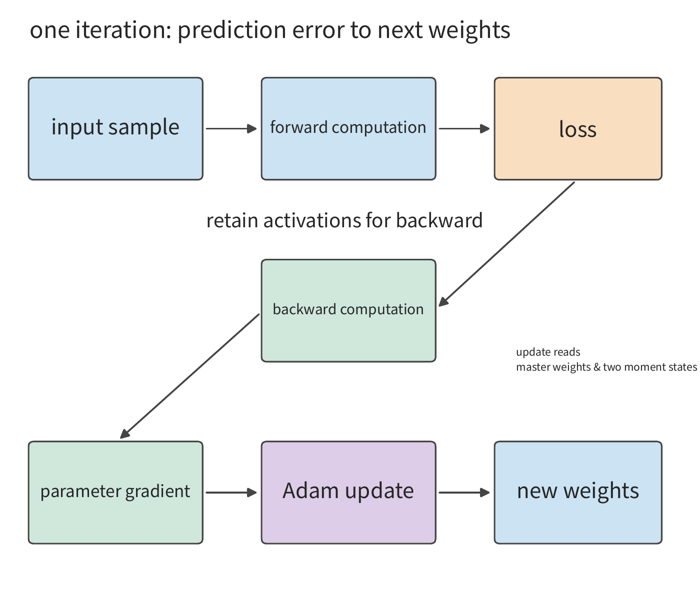
For the task in this chapter specifically, mixed-precision Adam performs matrix operations using BF16 weights, keeps FP32 master weights to hold the parameter values after the optimizer update, and keeps two FP32 moment states. The first and second moments are retained across iterations, recording the history of gradient direction and magnitude respectively; after the master weights are updated, they are converted back to BF16 for matrix operations. Gradients are accumulated in BF16. Summing term by term gives 16 bytes per parameter.

State	Bytes per parameter	Qwen3-8B capacity / GB	When used
BF16 model weights	2	16.4	Forward and backward matrix operations
BF16 gradients	2	16.4	Produced during backpropagation, used when computing new parameters
FP32 master weights	4	32.8	Store new parameters, then generate a BF16 copy
Adam first moment	4	32.8	Retains gradient history across training iterations
Adam second moment	4	32.8	Retains squared-gradient history across training iterations
Total	16	131.1	Persistent training state

Qwen3-8B has \(N=8\,190\,735\,360\) parameters, so

\[ M_{\mathrm{persistent}}=16N\approx131.1\ \mathrm{GB}\approx122.1\ \mathrm{GiB}. \]

Gradient format is another choice. Switching gradients to FP32 adds 2 bytes per parameter, bringing the total to 18 bytes. This change stems from the data format of the gradients; the term "mixed precision" itself does not dictate gradient format. MoE selects a subset of expert subnetworks via a router on each pass; each expert likewise has parameters and optimizer history to update, so the state capacity is determined by the total number of trainable parameters.⁷

Beyond how much space each category of data occupies, we must also distinguish how long each must be retained. Activations produced in the forward pass cannot be released until the corresponding backward computation finishes, while parameter-gathering buffers may be needed only during the execution of a particular module. The peak memory on card \(i\) depends on the training state, activations, and temporary buffers resident at the same instant:

\[ M_{\mathrm{peak},i}=\max_t\left[M_{\mathrm{persistent},i}(t)+M_{\mathrm{activation},i}(t)+M_{\mathrm{temporary},i}(t)\right]. \]

For example, if 8 GiB of activations and 4 GiB of gathering buffers appear at the same time, they jointly occupy 12 GiB; but if the activations are released before parameters are gathered, the same space can be reused. Capacity optimization thus has two directions: shrink the tensors and buffers themselves, or reduce how much data must be retained simultaneously. The sharding, recomputation, and offloading covered in the next section change the peak from each of these two directions respectively.

The capacity figures above assume matrix operations executed in BF16. Switching to a different floating-point format changes both the byte count of the state and the numerical risk. Consider FP16 first. Section 4.6.1 already compared the exponent and mantissa of FP16 and BF16: FP16's five-bit exponent puts the smallest normal number at \(2^{-14}\approx6.1\times10^{-5}\); values smaller than this can only be represented as subnormals, losing significant bits progressively as magnitude shrinks; values below \(2^{-24}\approx6\times10^{-8}\) become exactly zero. The mixed-precision training paper gives two sets of statistics: in the weight gradients of a Mandarin speech recognition model, about 5% of values have exponents below \(-24\) and would become zero in FP16, which the paper uses to argue for FP32 master weights; in the activation gradients of the Multibox SSD detection network, a large number of values fall below FP16's representable range and become zero, and among these, values in \([2^{-27},2^{-24})\) still matter for training.

Loss scaling solves this problem: before backpropagation, the loss is multiplied by a factor \(S\), scaling the gradients up by \(S\) times into FP16's representable range; before the parameter update, they are divided by \(S\) again. Across the various networks trained in that paper, the scaling factors used ranged from 8 to 32K. Too small a factor still lets small gradients underflow; too large a factor causes large gradients to overflow to infinity, requiring that update to be skipped and the factor reduced.²

BF16's eight-bit exponent matches FP32's, so the two share the same representable range and gradients need no scaling—this is one reason the state table above uses BF16. The cost is that the mantissa has only seven bits: the rounding error on matrix-operation inputs is larger than in FP16, and the precision of long inner products must be guaranteed by an FP32 accumulator.

Pushing the bit width lower still requires refining the single global scaling factor into block-wise scaling. FP8's E4M3 encoding has only four exponent bits and three mantissa bits, with a maximum normal value of 448; a single global factor cannot fit each layer's activations into such a narrow range simultaneously. DeepSeek-V3's FP8 training manages scaling by block: activations compute a scale per \(1\times128\) block (per token, per 128 channels), weights compute a scale per \(128\times128\) block, and the matrix unit converts partial sums to FP32 for continued accumulation every 128 elements accumulated. Compared with a BF16 control run, the relative loss error stays below 0.25%.²

FP8 also changes the capacity accounting, but only for the copy of the weights fed into the matrix unit: DeepSeek-V3's FP8 training converts the matrix-operation operands to FP8, while master weights, gradients, and optimizer state are still kept at higher precision. This FP8 operand copy costs 1 byte per parameter, plus one FP32 scale per \(128\times128\) block, totaling about \(1+4/16384\approx1.0002\) bytes per parameter; for Qwen3-8B, the weights read for matrix operations drop from BF16's 16.4 GB to about 8.2 GB, while the persistent training state of 16 bytes per parameter shown in the earlier table does not correspondingly drop to 1 byte.

Matrix-operation weight format	Bytes per parameter (incl. scale)	Weights read for Qwen3-8B matrix operations	Scale management	Main numerical risk
FP16	2	16.4 GB	Global loss scaling	Gradient underflow, scaling overflow
BF16	2	16.4 GB	Not needed	Shorter mantissa, compensated by FP32 accumulation
FP8 (E4M3) operand copy	~1.0002	~8.2 GB (master weights and optimizer state stored separately)	Block-wise scaling with periodic high-precision accumulation	Within-block rounding, stale scale

The lower the precision and the coarser the scaling granularity, the more capacity is saved, but the greater the risk of deviating from the high-precision reference. Whatever the cause—scaling failure, anomalous data, or hardware error—training divergence shows up as a spike on the loss curve, commonly handled by rolling back to the previous checkpoint and retraining. How much progress a rollback loses is determined by the save-period model in Section 10.4, and Section 10.4.5 further incorporates the rollback rate into that model.

10.1.3 Compute Requirements, MFU, and the Resource Lower Bound

Memory determines whether a model can begin training; compute speed determines whether it can finish on schedule. A model's state can be split across multiple cards, but how many cards are actually needed must be judged from the total computation and the deadline. One 8,192-token sequence requires about \(4.31\times10^{14}\) FLOPs of matrix computation across the forward and backward passes, averaging about 52.7 GFLOPs per token. Processing 100B tokens thus requires about \(5.27\times10^{21}\) FLOPs in total. This workload figure is accumulated from the model's matrix shapes and forward/backward operations.⁸

Suppose first that all 30 days are spent on training computation. The H100 SXM's dense BF16 matrix peak throughput is 989 TFLOP/s; at 40% of peak, one card processes about 7,500 tokens/s. Five cards together give about 37,600 tokens/s, below the roughly 38,600 tokens/s required for 30 days; at least six cards are needed to meet the compute requirement. By comparison, two 80 GB cards can already hold the 131.1 GB of persistent training state under ideal even splitting, yet would need about 77 days to finish the computation.

Let \(F\) be the total computation the algorithm requires, \(p\) the card count, \(P\) the peak throughput per card, and \(\eta\) the average compute efficiency over the measurement period. Then

\[ T=\frac{F}{pP\eta},\qquad p_{\mathrm{compute}}=\left\lceil\frac{F}{P\eta T_{\mathrm{available}}}\right\rceil. \]

This chapter computes MFU as defined in Section 1.2.2, with the denominator taken as the peak throughput of all cards. If the measured time is taken as the full training-iteration time, communication waiting is already included in it; if only the time the accelerator spends executing computation is counted, the result is the per-card compute efficiency. The design case in this chapter adopts the latter decomposition: per-card compute efficiency is taken as 40%, and then the communication time that cannot overlap with in-card computation, along with the time waiting for input data, are added on item by item. This makes it possible to directly observe the impact of each system design choice on completion time. The figure of 40% comes from Llama 3's public record: the 405B model was pretrained on 8,192 to 16,384 H100s with BF16 MFU of 38%–43%. That figure is computed over the full step time and thus already includes communication waiting; this chapter adds communication separately on top, so the completion time computed here runs somewhat longer. The RTX 4090 has no NVLink, so all inter-card data passes through PCIe; this cost is computed separately in Section 10.3.3 based on the actual link. Figures 10-3 through 10-5 also show the 30% and 50% brackets, to observe how card count changes as efficiency deviates.⁸

Where the remaining sixty percent of peak throughput goes is answered section by section in this chapter: communication that cannot overlap with computation (Section 10.3.3), pipeline bubbles (Section 10.3.2), memory-bandwidth-limited parameter updates and state conversion (Section 10.2.3), recomputation (Section 10.2.2), stragglers (Section 10.4.5), and checkpoint saving (Section 10.4.3). By the criterion in Section 1.3.4, the first four are work the model must account for—omitting any of them would make the estimated completion time too short—while the last two, along with the non-overlapped portion of communication, contain overhead that can be reduced; that is where the room for system-design optimization lies.

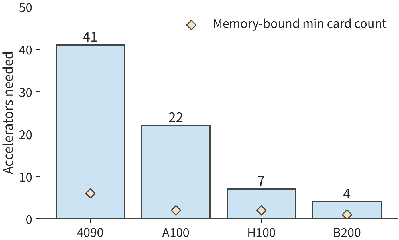
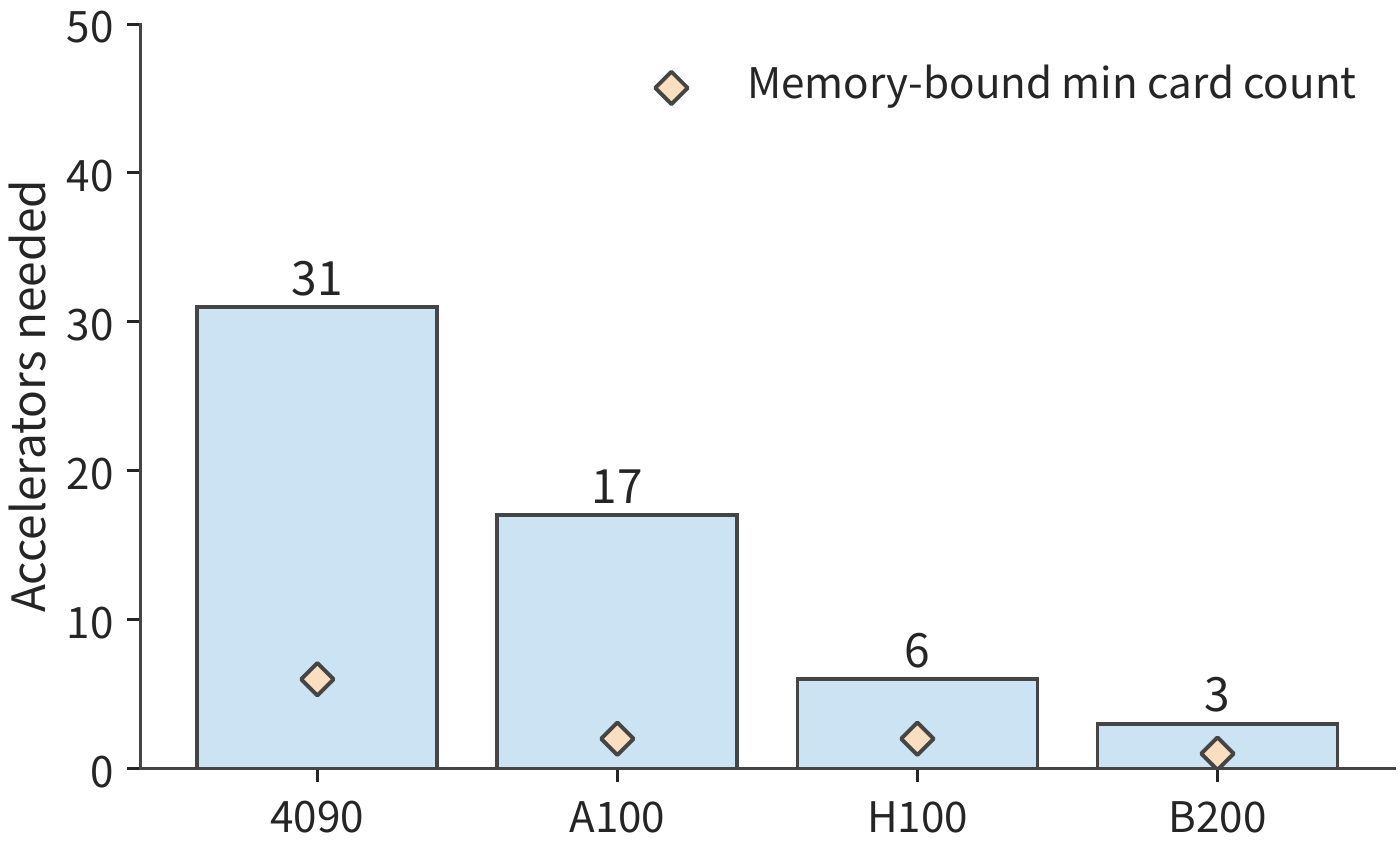
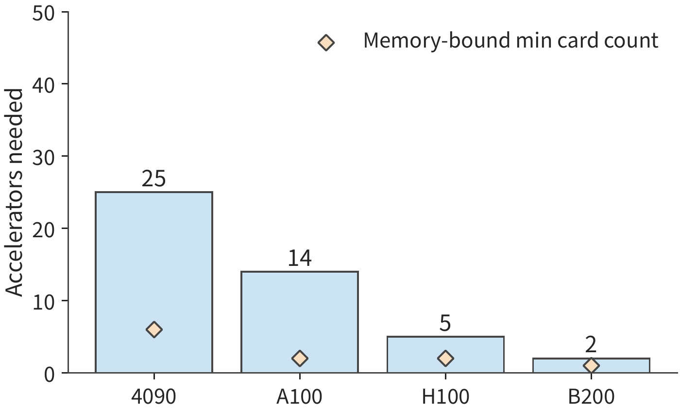
Figure 10-3 places the memory lower bound and the compute lower bound side by side: for the task in this chapter, the required card count is mainly determined by compute. Based on this, we now select two concrete configurations to compare step by step in later sections. The RTX 4090's corresponding peak is 165.2 TFLOP/s. At 40% efficiency and a 30-day deadline, at least 31 cards are needed. Adopting a configuration of eight cards per host, we can first consider a 32-card scheme; adding two more hosts gives 48 cards. In both schemes, each card accumulates 12 and 8 single-sequence micro-batches respectively, together completing a global batch of 384 sequences. Adding cards changes the work distribution, while the training objective stays the same.

Each training iteration involves about \(1.66\times10^{17}\) FLOPs. With 32 cards, each card takes about 78.3 s to complete its assigned computation; with 48 cards, about 52.2 s. Against the 67.9 s budget, the 32-card scheme is already over budget before communication is even added, while the 48-card scheme leaves about 15.7 s to spare. The next step is to determine how the two schemes organize their state, and which kinds of waiting will consume that 15.7 s.

10.2 Sharding, Recomputation, and Offloading of Training State

10.2.1 Data Parallelism and ZeRO/FSDP State Sharding

How state is distributed across multiple cards is determined by the parallelism strategy. Synchronous data parallelism has each card process different samples, then updates each card's own parameters using the reduced gradient. Since all cards end up with the same new parameters, each card typically keeps an identical copy of the weights and optimizer state; the more cards, the more redundant state. ZeRO was proposed by Microsoft researchers in 2019 and published in 2020; it uses cross-card sharding to reduce the redundant state copies kept during large-model training. ZeRO partitions ownership of this state in stages: each card is responsible for updating only part of the parameters, obtaining via communication whatever other data it needs for execution.

Fully Sharded Data Parallel (FSDP) organizes execution around the same sharding idea, with parameters, gradients, and optimizer state all sharded. Below, we use four cards to progressively change the ownership of state, then analyze the resulting execution pattern. In each figure, each column always corresponds to the same card; "full" means that card keeps the entire state, "shard" means it keeps only the quarter it is responsible for.

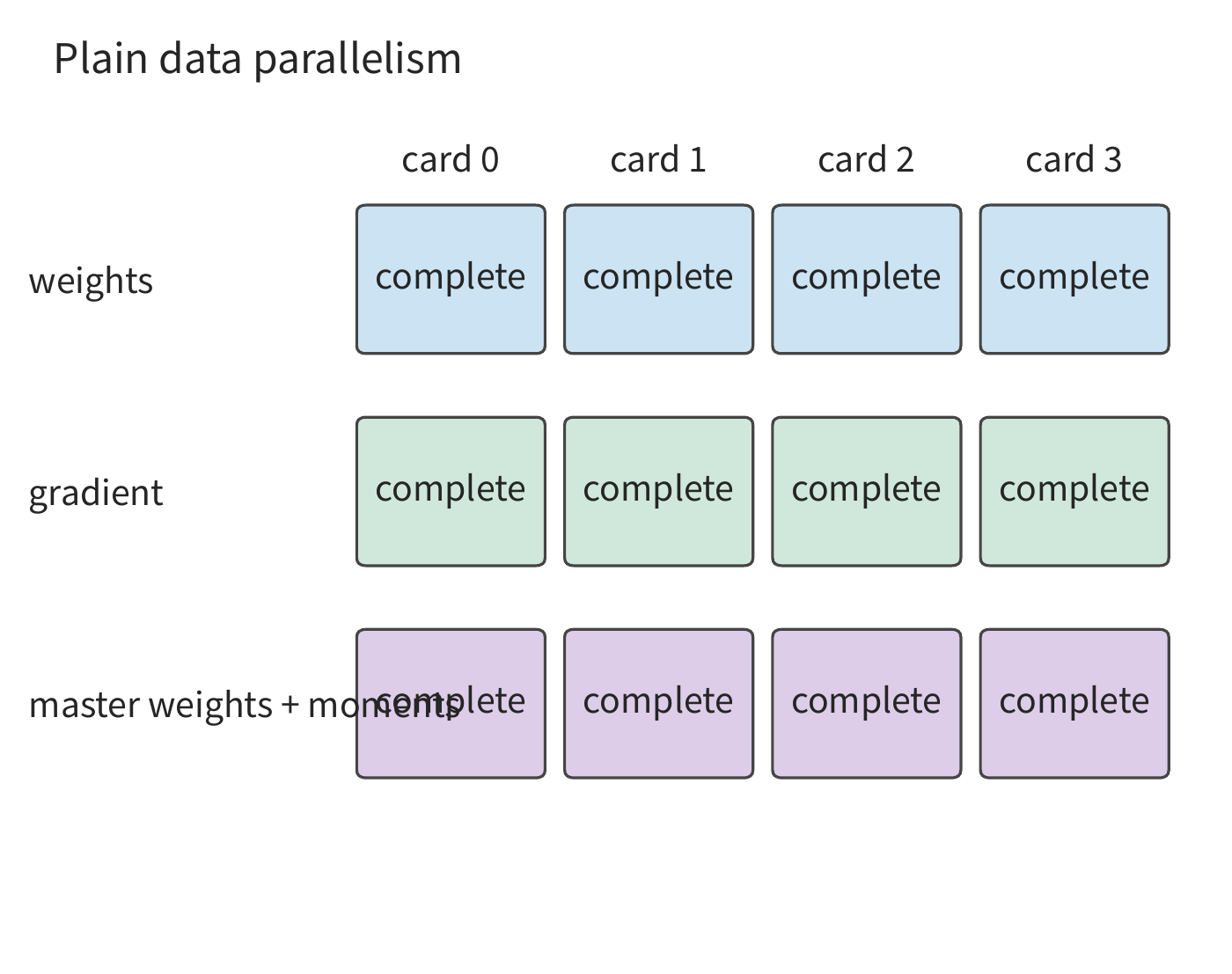
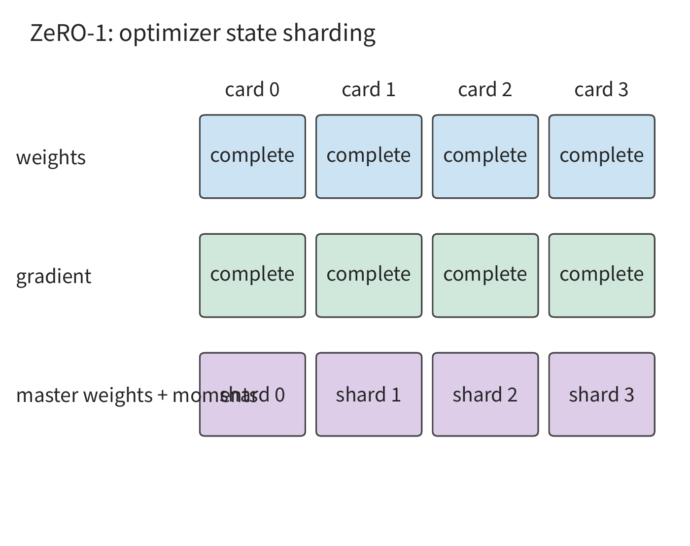
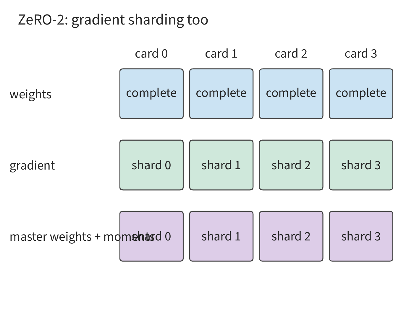
The first two stages still keep a full copy of the model weights on every card. Figure 10-9 partitions ownership of the weights as well, further reducing long-resident space, at the cost of needing communication to fetch the required weights before executing each module.

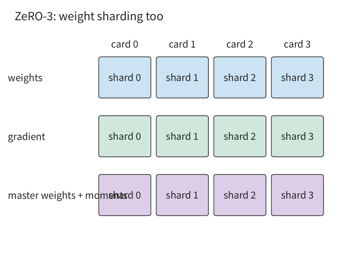
Let there be \(d\) cards in the data-parallel group. Computing the persistent training state first, the per-card capacities for plain data parallelism and the three ZeRO stages are

\[ \begin{aligned} M_0&=16N,\\ M_1&=4N+12N/d,\\ M_2&=2N+14N/d,\\ M_3&=16N/d. \end{aligned} \]

The first stage shards the FP32 master weights and the two Adam states, totaling 12 bytes/parameter, while weights and gradients are still each kept as one full copy. The second stage further shards the gradients, leaving only the BF16 weights fully replicated. The third stage shards the weights too. Substituting \(d=8\) gives the capacity changes shown below.

Configuration	Per-card persistent training state / GiB	Fully replicated training state
Plain DP	122.1	Weights, gradients, and optimizer state
ZeRO-1	42.0	Weights and gradients
ZeRO-2	28.6	Weights
ZeRO-3	15.3	All persistent training state sharded

Once sharded, each module executes in the following order: first gather the needed parameters via AllGather, perform the forward or backward pass, then aggregate gradients via ReduceScatter and distribute the gradient shards so that the card owning each shard receives its full gradient contribution, and finally each card updates the parameters it owns. FSDP's fully sharded execution is likewise organized around this path. If the full parameters are released after the forward pass, they must be gathered again before the backward pass; if they are kept, the backward pass can use them directly, but the full parameters then occupy memory alongside subsequent activations at the same time.

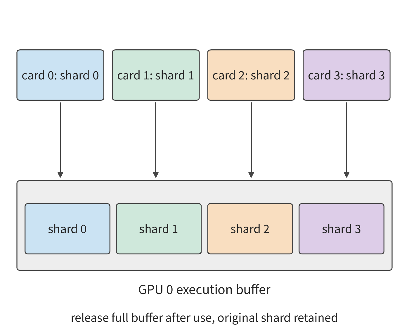
In Figure 10-10, the full-weight buffer coexists with the original shards. Increasing card count shrinks each original shard, but the size of the full-weight buffer is determined by the module itself. This is why the drop in persistent-state usage and the drop in execution peak differ in magnitude.

This difference can be observed directly in a small experiment. In one set of experiments using PyTorch's second-generation FSDP implementation (FSDP2) on a small CPU model, increasing the number of participating processes from two to four reduced the state retained after the parameter update from about 18 MiB to 9 MiB, while the execution peak dropped only from about 39 MiB to 30 MiB. The long-term-retained portion was halved, but the peak dropped only about 23%, because about 21 MiB of other tensors and buffers are still needed during execution. Analyzing the capacity requirements after sharding therefore also requires examining how long parameters and activations must be kept during module execution.⁹

10.2.2 Activation Retention and Selective Recomputation

The activations left behind by forward computation are like the intermediate steps recorded on scratch paper: when backward computation returns to this layer, some of those values are still needed. Keeping all the scratch work makes retrieval convenient but consumes space; keeping only some of the steps means the missing values must be recomputed before use. Parameter sharding has already reduced the duplication of weights and optimizer state; activation recomputation instead trades extra computation for the space needed to store these intermediate values.

Consider the matrix operation \(Y=XW\), where \(X\) is the input, \(W\) is the weight, and \(Y\) is the output. After forward computation finishes, \(X\) still needs to wait until the weight gradient is computed. Let the loss be \(\mathcal L\), let \(dY=\partial\mathcal L/\partial Y\) be the gradient passed in from downstream computation, and let \(dX\) and \(dW\) be the gradients of the loss with respect to the input and the weight, respectively; the superscript \(\mathsf T\) denotes matrix transpose. The backward pass computes

\[ dX=dY W^{\mathsf T},\qquad dW=X^{\mathsf T}dY. \]

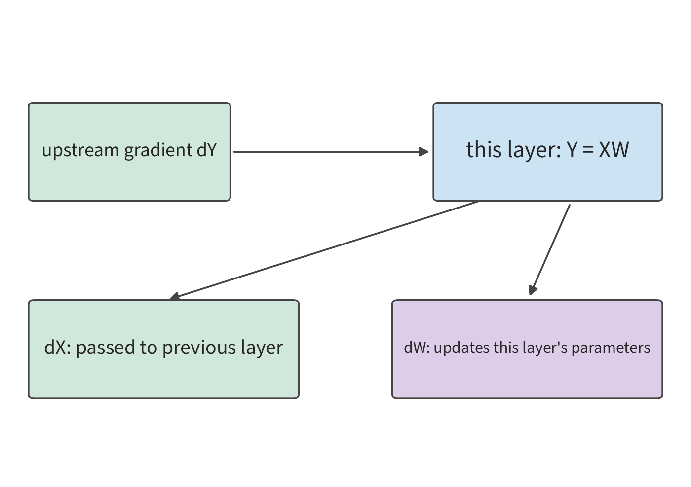
Computing the parameter gradient requires the forward input \(X\). If \(X\) is retained, it must stay resident from forward computation until backward computation finishes using it; if \(X\) is released, the corresponding forward computation must be re-executed before backward use, starting from the retained inputs or intermediate results. Which values to keep and which to recompute depends on how much space is saved and how much work recomputation requires.

Example: How much activation storage does recomputing the gate product save before backward propagation? The MLP (multi-layer perceptron, the feedforward subnetwork in this example) of Qwen3-8B first computes the gate result \(a\) and the up-projection result \(u\), then forms \(h=a\odot u\), and finally computes \(Y=hW_{\mathrm{down}}\). The parameter gradient for the down-projection requires \(h\). If \(a,u\) are already retained for the backward computation of the nonlinear operator, they can be re-multiplied right before the down-projection's backward pass, so \(h\) does not need to be retained the whole time.

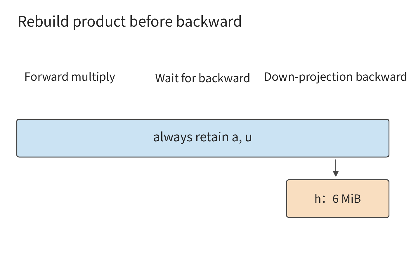
After rebuilding, h only needs to be generated right before the down-projection's backward pass begins, and retained until that computation finishes. The size of this buffer is as follows: for a 128-token micro-batch with FP32 activations, \(h\) has shape \([128,12288]\), occupying \(128\times12288\times4=6\) MiB; rebuilding it requires about 1.57 million multiplications. The two normalized weighted outputs in the same layer both have shape \([128,4096]\), each occupying 2 MiB, and can likewise be rebuilt from the saved normalized results and weights. This saves \(6+2+2=10\) MiB per layer, and 90 MiB per micro-batch across a nine-layer pipeline stage, roughly 94 MB.

In the original scheme, the inputs saved for these GEMMs occupy 15 MiB per layer, of which the three products above account for 10 MiB, and Q, K, V, and the attention output account for the remaining 5 MiB. The nine-layer stage thus drops from 135 MiB to 45 MiB, that is, from roughly 142 MB to 47 MB. The rebuilding happens layer by layer in sequence; the largest product's working buffer is 6 MiB, and once one layer finishes using it, the next layer reuses the same space.¹⁰

If four micro-batches are simultaneously waiting for backward computation, the data that must be retained long-term drops by \(4\times90=360\) MiB, roughly 377 MB, with the rebuild computation then performed micro-batch by micro-batch during backward. The benefit here comes from the difference in data lifetimes: the more micro-batches waiting for backward computation, the more data must be retained long-term; when rebuilding layer by layer, however, the same working buffer can be reused repeatedly. If pipeline scheduling causes backward computation to start earlier, the number of micro-batches waiting for backward computation drops accordingly. Recomputation and pipeline scheduling therefore jointly determine how much data must be retained; whether the added computation lengthens per-step training time depends on where it sits on the timeline.

10.2.3 CPU/GPU Offloading and Buffer Usage Time

When the cost of rebuilding data from saved results is small, recomputation is a good fit. Another approach is to keep the data itself but move it to host memory, which has larger capacity, and transfer it back to the GPU before use — this is offloading. Once offloading is chosen, the original GPU memory problem becomes a question of whether the transfer can complete in time. Suppose a piece of state has size \(V\), the link's effective bandwidth is \(B\), and there are \(W\) seconds between when the transfer can start and when the operator needs this data; then the transfer time exceeding this window is

\[ T_{\mathrm{wait}}=\max(0,V/B-W) \]

and the corresponding operator must wait this long. How much the transfer and computation can overlap depends on when the data can be sent, when the link is free, and when the corresponding operator needs the data. DMA transfers are initiated by the device, and the source data must remain valid throughout the transfer. The source buffer stays valid until the DMA completes, and the destination buffer occupies memory from the moment it starts receiving data; offloading changes the usage time of buffers at both ends simultaneously.

Example: Converting gradients on CPU or GPU — which completes offloading faster? The gate-projection gradient has shape \([12288,4096]\); its BF16 size is \(G=96\) MiB, and its FP32 size is 192 MiB. CPUAdam is an implementation that runs the Adam update on the CPU; it uses FP32 gradients, so it can either transfer BF16 first and convert on the CPU, or convert on the GPU first and then transfer FP32. Either conversion reads \(G\) and writes \(2G\), accessing \(3G\) bytes in total. The conversion is limited by memory bandwidth: for the GPU we take the RTX 4090's 1008 GB/s, and for the CPU we take the fourth-generation Xeon single-socket eight-channel DDR5-4800's 307.2 GB/s. Let \(C_c,C_g\) denote CPU and GPU conversion throughput, and let \(B\) be the link's effective bandwidth; the serial path times are

\[ T_c=G/B+3G/C_c,\qquad T_g=3G/C_g+2G/B. \]

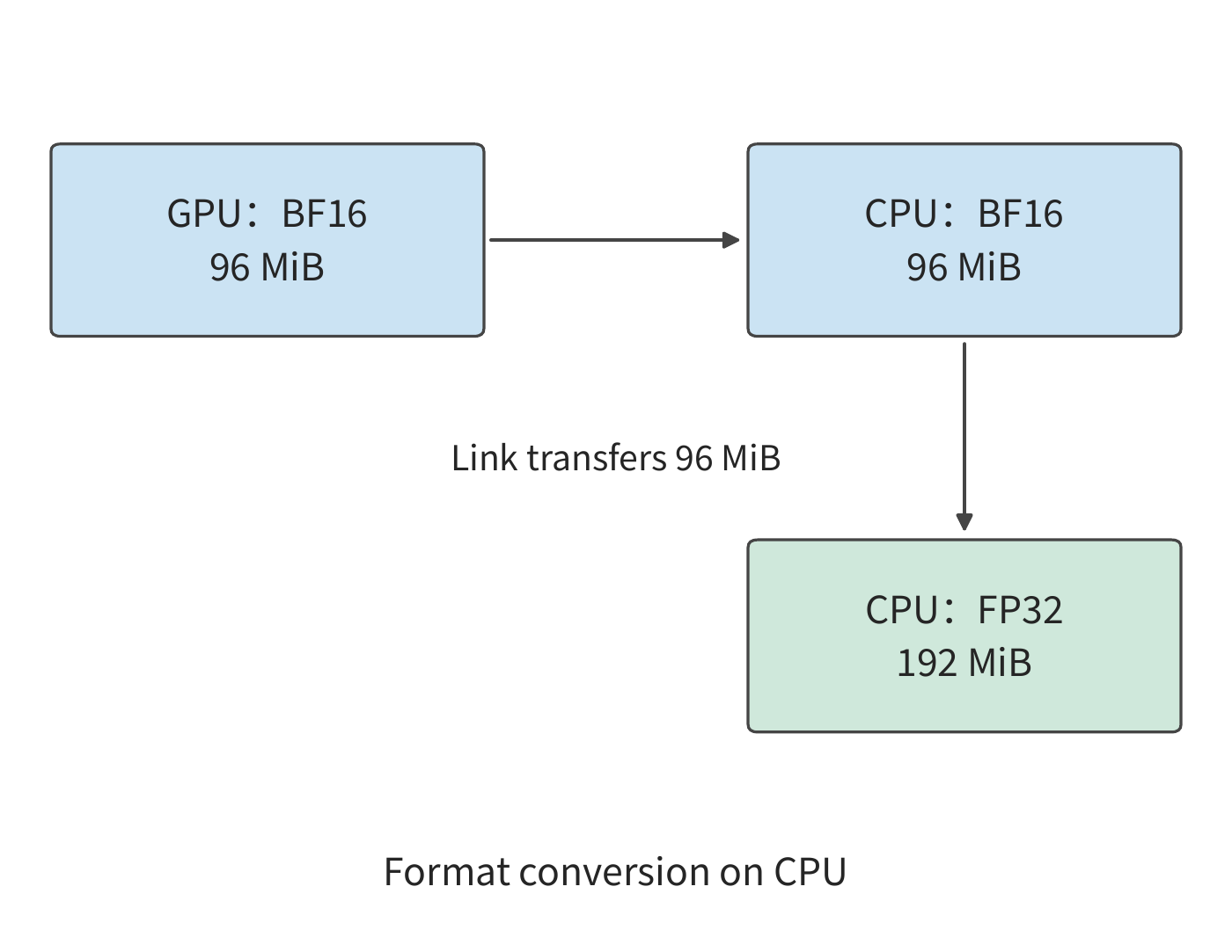
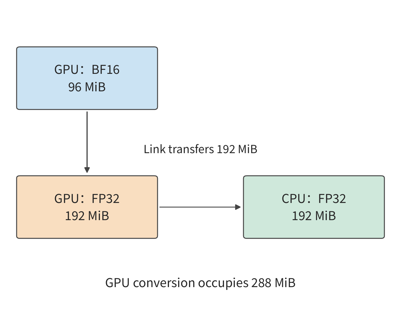
The difference between Figure 10-14 and Figure 10-15 centers on the arrow crossing the link: although the GPU converts faster, it must transfer 96 MiB more. The slower the link, the more easily this extra transfer offsets the conversion benefit.

The RTX 4090 connects to the host via PCIe 4.0 x16, at 32 GB/s in each direction. On this link, the CPU path takes about \(3.15+0.98=4.13\) ms, and the GPU path takes about \(0.30+6.29=6.59\) ms. The GPU path's conversion is about 0.68 ms faster, but its transfer is about 3.15 ms slower, making it slower overall. If the link is instead the NVLink-C2C between CPU and GPU in a GH200, at 450 GB/s in each direction, the extra 96 MiB transfer only adds about 0.22 ms; the two paths become about 1.21 ms and 0.75 ms, and GPU conversion gains a clear advantage.¹¹

Setting the two path times equal gives the bandwidth threshold at which the faster method switches:

\[ B^*=\frac{1}{3(1/C_c-1/C_g)}\approx147\ \mathrm{GB/s}. \]

This threshold places two opposing effects on the same scale: GPU conversion is faster, saving format-conversion time; FP32 data is larger, adding transfer time. The faster the link, the smaller this latter cost. Since 147 GB/s exceeds PCIe 5.0 x16's 64 GB/s per direction, cards connected via PCIe should, in this example, always transfer BF16 first and convert on the CPU.

GPU memory capacity introduces another constraint. During GPU conversion, the original 96 MiB and the output 192 MiB coexist, for a peak of 288 MiB; the path that transfers BF16 first only needs to retain the 96 MiB gradient involved in that conversion on the GPU. Choosing GPU conversion requires an extra 192 MiB buffer. SuperOffload is a training offload system for tightly coupled CPU-GPU chips like the GH200; it schedules the conversion location together with optimizer execution on the host, exploiting exactly this trade-off among conversion speed, transfer data volume, and buffer usage time. The overall step's benefit is then determined by when the last gradient bucket, the CPU-side parameter update, and the weight transfer back all complete.

10.2.4 Per-Card State Allocation and Interconnect Topology in Combined Parallelism Schemes

Sharding, recomputation, and offloading change storage, computation, and transfer volume, respectively. When combining these approaches into a complete system, one must also determine which cards and communication groups they act on. The parallelism methods in Chapters 6 and 7 partition different data and computation during training: TP splits within-layer matrices, PP partitions layers, DP partitions samples, and EP partitions experts. The overview table in Section 6.1.4 also includes SP and CP: the former shards the activations of per-token operators along the sequence, usually reusing the tensor-parallel group; the latter distributes the attention context of the same long sequence across multiple cards, preserving cross-position dependencies. These parallelism methods extend the "tile — arrange inputs — merge results" approach from Chapter 5, with training then propagating gradients backward along the same computation graph. By first determining who updates each parameter, then arranging collection, exchange, and reduction along the forward and backward dependencies, one obtains both per-card capacity and traffic at each interface simultaneously.

Three capacity optimizations can be compared using the same set of questions.

Method	Memory footprint reduced	Extra work added	Timing relationship determining benefit
State sharding	Duplicated weights, gradients, or optimizer state	Parameter gathering, gradient reduction and sharding	Whether gathering finishes in time before the module executes
Activation recomputation	Intermediate values held from forward to backward	Rebuilding forward values	Whether rebuilding delays backward computation on the critical path
State offloading	State temporarily unused on the accelerator	Transfer between host and accelerator	Whether the data transfers back before use

Example: When GPU memory is insufficient, should you increase the number of sharding participants or recompute activations? The RTX 4090 is nominally rated at 24 GB, about 22.35 GiB; after subtracting runtime overhead, we count 22 GiB of usable GPU memory per card. Qwen3-8B with ZeRO-3 on eight cards retains about 15.3 GiB per card, leaving about 6.7 GiB for other tensors and buffers. If activations and temporary buffers simultaneously need 10 GiB, the total is about 25.3 GiB, exceeding the budget by about 3.3 GiB. At this point, one can use recomputation to save this 3.3 GiB, or scale up to sixteen cards, lowering the resident training state to about 7.6 GiB, bringing the total down to about 17.6 GiB.

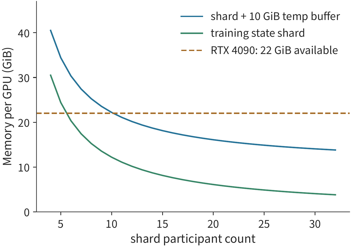
The two choices correspond to different costs: the eight-card scheme adds rebuild computation, while the sixteen-card scheme adds cards and changes the communication group. One can first identify from the figure which schemes satisfy the memory requirement, then compare the per-step time of these schemes.

For the training task in this chapter, both the 32-card and 48-card schemes use full-group ZeRO-3, with TP=PP=1, and each card's micro-batch is a single sequence. As in the previous example, we count 22 GiB of usable GPU memory per card, and budget 10 GiB for the simultaneously retained activations, complete module parameters, and working buffers. The resident training state of the two schemes is about 3.8 and 2.5 GiB respectively, for totals of about 13.8 and 12.5 GiB, with capacity margins of about 8.2 and 9.5 GiB. GPU memory is sufficient for both schemes, so the comparison now turns mainly to completion time.²⁷

10.3 Pipeline Scheduling and Communication Overlap Within a Training Step

Capacity analysis determines whether GPU memory can hold the required data; timing analysis determines whether the data arrives in time. This section first clarifies the objective function optimized in one training iteration, then places forward computation, backward computation, and communication on the same timeline. The design case in this chapter uses data parallelism; a four-stage pipeline serves as a standalone example, illustrating how scheduling simultaneously changes both the critical path and activation lifetimes.

10.3.1 Micro-batches, Gradient Accumulation, and Parameter Updates

The global batch contains all the samples used for one parameter update, and can be split into multiple micro-batches that execute backward propagation in sequence, accumulating gradients before a unified update. Let the index set of valid tokens in micro-batch \(k\) be \(S_k\), let the total number of valid tokens be \(L=\sum_k|S_k|\), and let the average per-token loss be

\[ \mathcal L=\frac{1}{L}\sum_k\sum_{j\in S_k}\ell_j. \]

Summation and differentiation can be swapped, so backward propagation can be executed separately for each micro-batch; when computing the loss for each micro-batch, its loss sum is divided by the same \(L\) each time. Once the gradients from all micro-batches have accumulated, one gradient clipping step and one parameter update are performed. Splitting into micro-batches this way changes only the execution order, not the weight each token carries in the loss function.

Example: Why does averaging by micro-batch versus by token change the gradient? Among eight responses, four each contain two valid tokens and four each contain three, totaling 20. Let the per-token loss of a short response be \(\theta/5\) and that of a long response be \(2\theta/5\); then

\[ \mathcal L=\frac{8\theta/5+12(2\theta/5)}{20}=\frac{8\theta}{25},\qquad \frac{d\mathcal L}{d\theta}=0.32. \]

If we first compute the average loss of each response, then average over the eight responses, short and long responses each carry half the weight, and the gradient becomes \((0.2+0.4)/2=0.30\). Under the original per-token averaging, long responses account for \(12/20=60\%\), so the result leans closer to 0.4. If the common denominator of 20 has already been applied, and the accumulated result is divided by eight again, the gradient becomes 0.04. The denominator determines each token's contribution to the parameter gradient.²⁰

Back to the design case: the 384 full-length sequences from Section 10.1.3 accumulate 12 micro-batches per card on 32 cards, and 8 micro-batches per card on 48 cards. Each card processes one sequence at a time, and every card executes the same matrix shapes; the global count of valid tokens and the objective function are also the same. Parameter gathering and gradient communication are then separately scheduled onto the timeline according to the execution path.

10.3.2 Pipeline Scheduling, Bubbles, and Activation Lifetimes

Splitting into micro-batches preserves the training objective but changes the order in which computation happens. In pipeline parallelism, this order also determines when each stage can start computing and how many copies of activations are waiting for backward computation. Pipeline parallelism splits the model into multiple stages, with each micro-batch proceeding forward in sequence and then propagating gradients backward. Fill-drain scheduling completes the forward pass of all micro-batches first, then executes the backward pass in a concentrated block. 1F1B (one forward, one backward) alternates one forward and one backward pass after the pipeline warms up, letting earlier micro-batches release their activations sooner.

How quickly activations are released directly determines the memory peak. Backward computation needs the activations saved during the forward pass, so each micro-batch's activations must stay in memory from the moment forward computation finishes until the corresponding backward pass arrives. However many micro-batches are simultaneously waiting for backward computation, that many copies of activations sit in memory. Fill-drain must wait for all \(m\) micro-batches to finish forward computation before starting the first backward pass, so the peak grows linearly with \(m\); once it exceeds memory capacity, this training step cannot execute at all, and one can only reduce the number of micro-batches concurrently in the pipeline, shorten the sequence, or switch to more expensive recomputation to make it feasible. Executing backward computation earlier means ending the activation's waiting period sooner: once the peak drops, the training step becomes feasible, or the freed-up margin can go toward larger micro-batches and longer sequences. Memory residency is thus often not a question of speed but of whether execution is even possible.

Comparing any two scheduling schemes requires examining two axes at once: one is completion time, determined by the size of idle waiting (bubbles) in the pipeline; the other is memory residency, determined by how long each activation must be retained before its corresponding backward pass arrives.

Suppose first that \(p\) stages are perfectly balanced, with forward time \(t_f\) and backward time \(t_b\) per stage, and transfer and parameter-update time taken as zero. Filling and draining \(m\) micro-batches requires

\[ T=(m+p-1)(t_f+t_b),\qquad u=\frac{m}{m+p-1}. \]

The \(m\) term here corresponds to the actual computational work of the micro-batches, while the \(p-1\) term comes from filling and draining. The utilization \(u\) therefore rises as the number of micro-batches increases. Taking \(p=4,m=8\) gives \(u=8/11\approx72.7\%\). If the global batch size is kept fixed, increasing the number of micro-batches means shrinking each one; the resulting reduction in pipeline idle time must be weighed against the execution time of these smaller matrices.

Example: With the same bubble, what does 1F1B buy? Split the 36 layers of Qwen3-8B into four nine-layer stages, with eight micro-batches, each containing one 128-token sequence. Each stage's forward pass takes 10 ms, backward pass takes 20 ms, boundary transfer takes 1 ms each way, forward and backward links are independent, and parameter update takes 1 ms. Fill-drain scheduling without transfer takes \((8+4-1)\times30=330\) ms; forward filling across three boundaries adds 3 ms, backward draining adds another 3 ms, and the parameter update adds 1 ms, for a total of 337 ms.

1F1B starts backward computation earlier, so subsequent forward passes must then wait for backward computation to free up compute resources. At stage 0, the first four micro-batches finish forward computation at 40 ms, and the first returned gradient arrives at 106 ms. Backward computation then runs until 126 ms, at which point the fifth micro-batch begins its forward pass. This interleaving cascades downstream arrival times level by level. Stage 3 finishes the backward pass of the second micro-batch at 93 ms, but the third forward input does not arrive until 95 ms, producing a 2 ms gap; subsequent similar waits continue to lengthen the critical path. After scheduling the execution order according to these dependencies, all gradients finish computing at 346 ms, and with the parameter update, the total is 347 ms.¹⁰

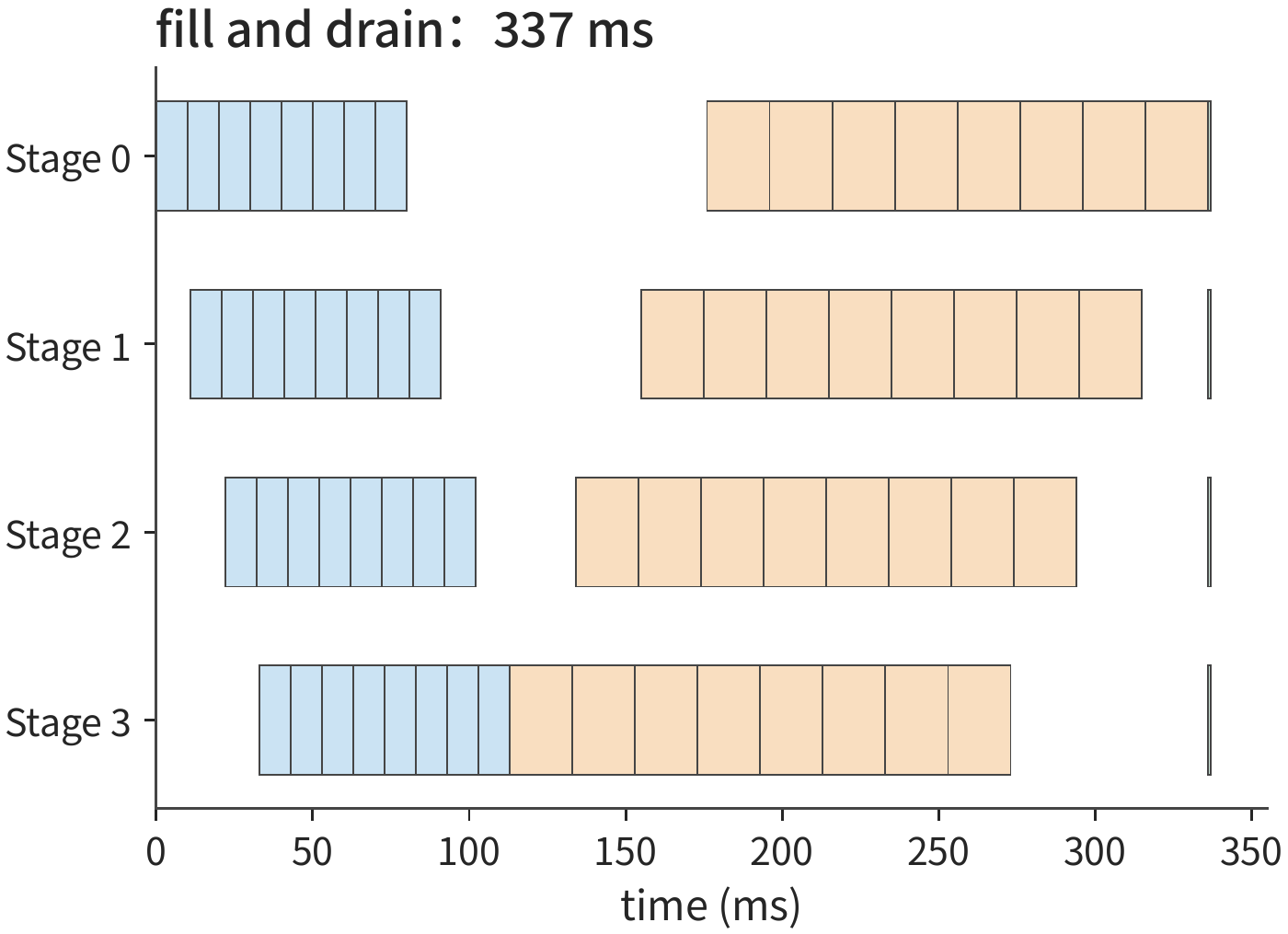
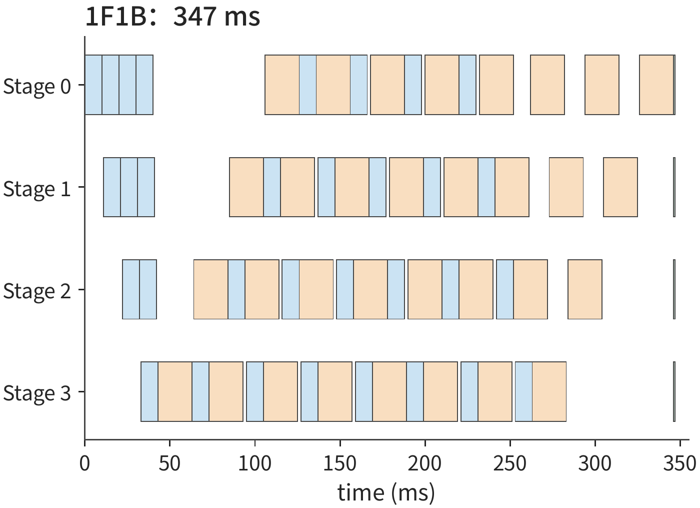
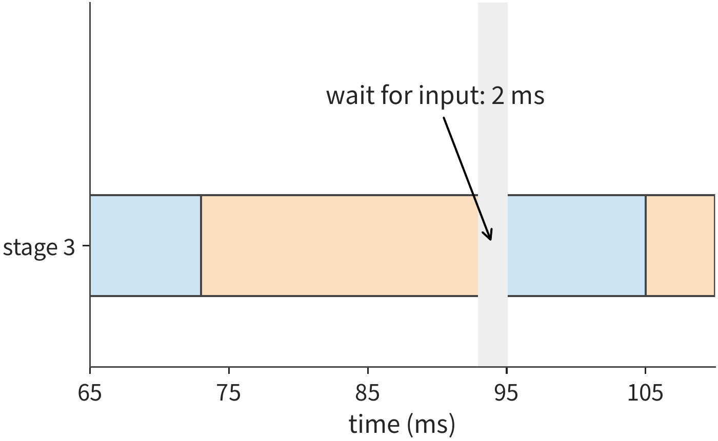
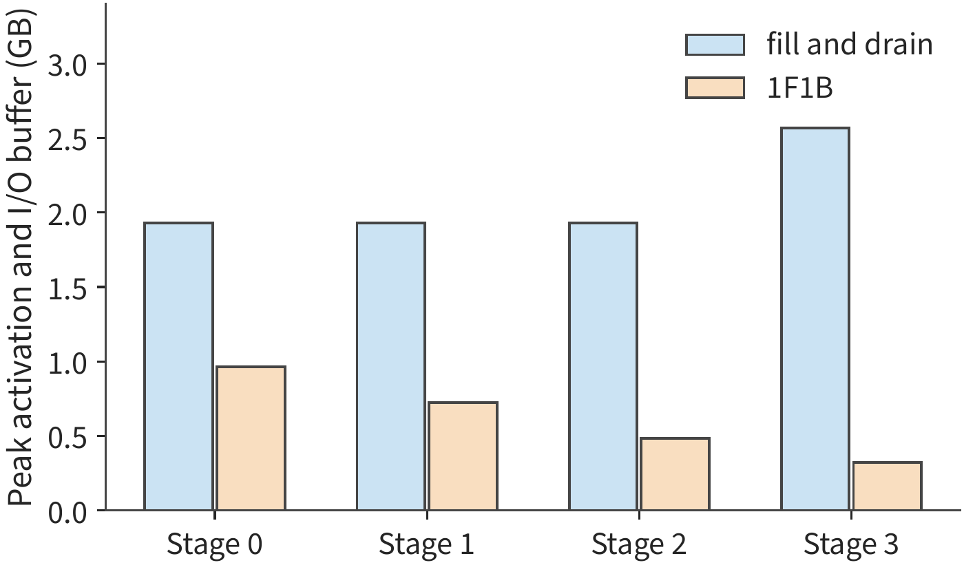
Comparing the two figures shows that both schedules perform the same forward and backward work, and the bubble time is the same \((p-1)(t_f+t_b)\) in both; 1F1B, because of the dependency waits introduced by interleaving (Figure 10-19), actually takes about 3% longer, but the benefit shows up in Figure 10-20 — the peak memory usage of intermediate results and buffers drops from about 2.57 GB to 0.97 GB, a reduction of about 62%. So "1F1B is better than fill-drain" only holds on the memory axis; on the time axis it is actually slightly slower. If only 1 GB is budgeted for these intermediate results and buffers, only the earlier-backward schedule can execute this training step; when capacity is ample, the 337 ms fill-drain schedule finishes sooner. Which schedule to choose is determined jointly by "when tensors are released" and "when the next input becomes available."

To shorten completion time, the bubble itself must be compressed: splitting backward computation more finely and keeping more micro-batches flowing simultaneously fills the gaps more completely. The three classes of scheduling below all build on the dependency analysis above, trading communication count, activation peak, and parameter count, respectively, for a smaller bubble. All three use the same example (four stages, 10 ms forward, 20 ms backward, 1 ms boundary transfer, 1 ms parameter update); the execution order of each micro-batch at each stage (slot order) is scheduled by an event model, and the bubble formulas and backward-splitting ideas come from published papers.³

Interleaved 1F1B (also called virtual pipelining) cuts the 36 layers into eight blocks, distributed round-robin across four cards, giving each card \(v=2\) non-contiguous blocks, totaling nine layers as before: the first four blocks each have five layers, the last four each have four layers; card 0 executes layers 0–4 and layers 20–23, and the rest follow similarly. Each micro-batch's forward pass therefore crosses \(2p-1=7\) boundaries instead of 3, and the bubble ratio shrinks from \((p-1)/m\) to

\[ \frac{1}{v}\cdot\frac{p-1}{m}. \]

With eight micro-batches, completion time drops from 347 ms to 298 ms, and per-card idle time drops from about 106 ms to about 57 ms. There are two costs: the number of transfers more than doubles (the full step's forward messages increase from 24 to 56), and earlier stages' activations must wait for more blocks to finish forward computation — stage 0's peak activation and send/receive buffer usage rises from 921 MiB to about 1,329 MiB.

Zero-bubble scheduling splits backward computation into two parts: the input gradient \(dX\) (denoted B in the paper) must be passed to the previous stage, which is waiting for it, so \(dX\) sits on the critical path and should execute as early as possible; the weight gradient \(dW\) (denoted W in the paper) only feeds into this layer's gradient accumulation and can be placed at any time after this stage's corresponding \(dX\), so it is deferred to fill gaps. Let the per-stage times for forward, \(dX\), and \(dW\) be \(T_F\), \(T_B\), and \(T_W\) respectively; then 1F1B's bubble is \((p-1)(T_F+T_B+T_W)\); ZB-H1 fills \(dW\) into the gaps, reducing the bubble to \((p-1)(T_F+T_B-T_W)\); ZB-H2 moves more forward passes earlier, reducing the bubble to \((p-1)(T_F+T_B-2T_W)\). The zero-bubble paper's two hand-crafted schedules are constructed with \(T_F=T_B=T_W\); Table 2 of the paper gives the general form above.

In this example, split the 20 ms backward pass evenly into \(T_B=T_W=10\) ms: 1F1B's bubble is \(3\times30=90\) ms, ZB-H1's lower bound is \(3\times(10+10-10)=30\) ms, and ZB-H2's lower bound is 0. Scheduling events according to the ZB-H1 slot order in Figure 3 of the paper, the eight micro-batches complete in 283 ms, with 42 ms of per-card idle time; setting boundary transfer to zero, the idle time is exactly the 30 ms lower bound, with the extra 12 ms coming from transfer. Stage 0's peak activation and send/receive buffer usage is the same as 1F1B's, 921 MiB. The cost falls on later stages: stage 3's \(dW\) executes three micro-batches later than its \(dX\), and the event model retains a full copy of the activation during this period, raising stage 3's peak from 1F1B's 308 MiB to about 1,226 MiB. The paper computes this using the smaller activation amount actually needed for \(dW\), and its Table 2 gives ZB-H1's peak as the same \(pM_B\) (\(M_B\) being the activation amount of one micro-batch) as 1F1B.

DualPipe splits micro-batches into two halves, injecting them from both ends of the pipeline toward each other, so each stage simultaneously carries blocks from both directions. Following DeepSeek-V3's notation, its bubble is \((PP/2-1)(F\&B+B-3W)\), where \(PP\) is the number of pipeline stages, \(F\&B\) is the period during which forward and backward computation overlap, \(B\) denotes the full backward pass of 20 ms, and \(W\) denotes its \(dW\) portion of 10 ms. This example does not simulate overlapping forward and backward computation, taking \(F\&B=F+B=30\) ms, giving a bubble of \((2-1)\times(30+20-30)=20\) ms and a completion time of 306 ms. The cost is equally direct: each card must store parameter copies for both directions, doubling the parameter count, and activations are retained for \(PP+1\) copies; in this example, per-stage peaks are about 1,228–1,612 MiB.³

The table below places these five schedules side by side under the same example. Fill-drain, despite not compressing the bubble, remains the baseline when capacity is ample, and is listed alongside the others:

Schedule (eight micro-batches)	Completion time / ms	Per-card idle time / ms	Stage 0 peak / MiB	Bubble-compression mechanism	Main cost
Fill-drain	337	96	1,840 (stage 3: 2,448)	None	Highest activation residency; infeasible when capacity is tight
1F1B	347	106	921	None (same bubble as fill-drain)	Cheapest on memory, but about 3% slower than fill-drain
Interleaved 1F1B, \(v=2\)	298	57	1,329	Per-card layer blocks split into \(v\) segments	Forward messages increase from 24 to 56
Zero-bubble (ZB-H1), \(T_B=T_W\)	283	42	921 (stage 3: 1,226)	\(dW\) deferred to fill gaps	Later stages' activations must be retained until \(dW\) executes
DualPipe	306	65	1,228 (stages 1, 2: 1,612)	Micro-batches flow from both ends toward each other	Two copies of parameters per card

Plotting the numbers from the table onto each stage's timeline shows exactly where the bubbles get filled in. The three figures below use the same timescale and colors as Figures 10-17 and 10-18.

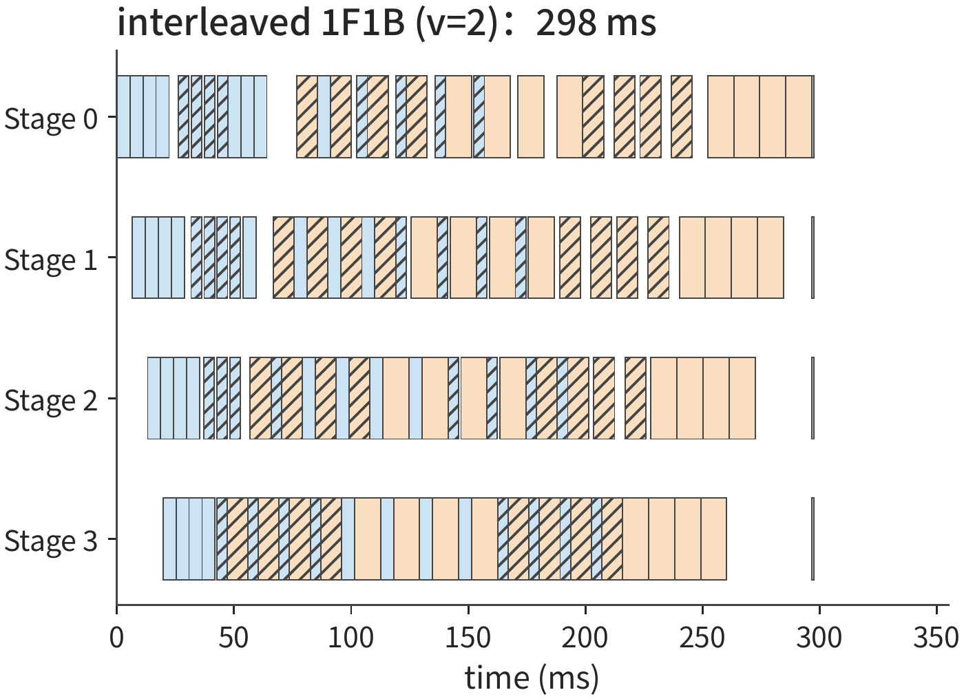
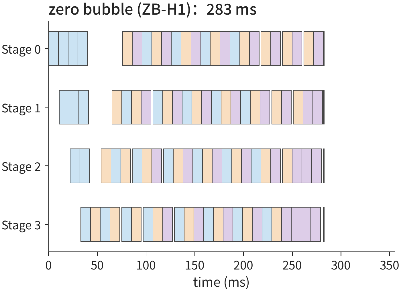
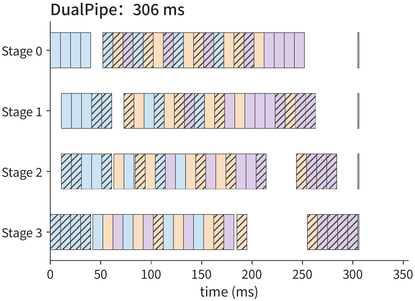
No single schedule dominates on both axes. Ranking the five schedules separately along each axis gives a different winner each time: zero-bubble has the shortest completion time, while 1F1B has the lowest maximum single-stage peak. The time saved by the three extended schedules' bubble compression each comes at the cost of increasing some other resource, so choosing a schedule requires first determining which side the constraint falls on: time or capacity. Figure 10-24 plots both axes side by side (fill-drain is not plotted), for comparison against the table above.

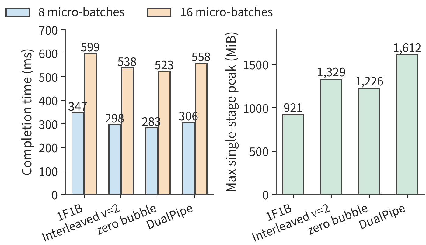
When the number of micro-batches doubles to 16, the completion times for 1F1B, interleaved, zero-bubble, and DualPipe are 599, 538, 523, and 558 ms respectively, with the same ranking as before. Whether compressing the bubble is worthwhile depends on the relative size of the bubble time saved versus the added cost. As \(m\) grows, the bubble ratio \((p-1)/m\) itself keeps falling — at 16 micro-batches, 1F1B's bubble fraction has already dropped from 37.5% to 18.8%, so the relative benefit of finer splitting shrinks accordingly, while interleaved's added communication count, zero-bubble's added activation residency, and DualPipe's added parameter count do not shrink with \(m\). The link contention discussed in Section 10.3.3 provides another boundary: the four extra cross-boundary transfers that interleaved adds per micro-batch will directly lengthen the critical path when the link is already saturated by gradient reduction. When capacity is tight, the order of selection reverses: first eliminate schedules that are infeasible on peak usage per Section 10.2.4, then compare completion times.

10.3.3 Backward Dependency, Gradient Bucketing, and Communication Overlap

The 2 ms gap in the previous section came from input not yet having arrived. Gradient communication is governed by the same rule: sending must wait for data to be produced, and once sending begins, it must also wait for the link to be idle. Backpropagation produces gradients layer by layer; implementations typically merge multiple gradient tensors into a single communication bucket and send it only after all gradients within the bucket have been computed. The larger the bucket, the more likely it is to wait for the gradient produced last; the smaller the bucket, the more times communication must be launched. Scheduling must balance launch cost against sending early.

Suppose a reduction requires 3 ms, and after the gradient is ready there is 5 ms of unrelated computation, during which the reduction can proceed concurrently. If the shared link has already scheduled 4 ms of expert exchange beforehand, the reduction can only use the remaining 1 ms, leaving 2 ms that extends past the end of the computation. This portion, which cannot overlap with computation and extends the training step, is called communication wait time. Data dependency determines the earliest possible start time, resource contention pushes it later, and the dependencies of subsequent operators determine whether this wait extends the entire training step.

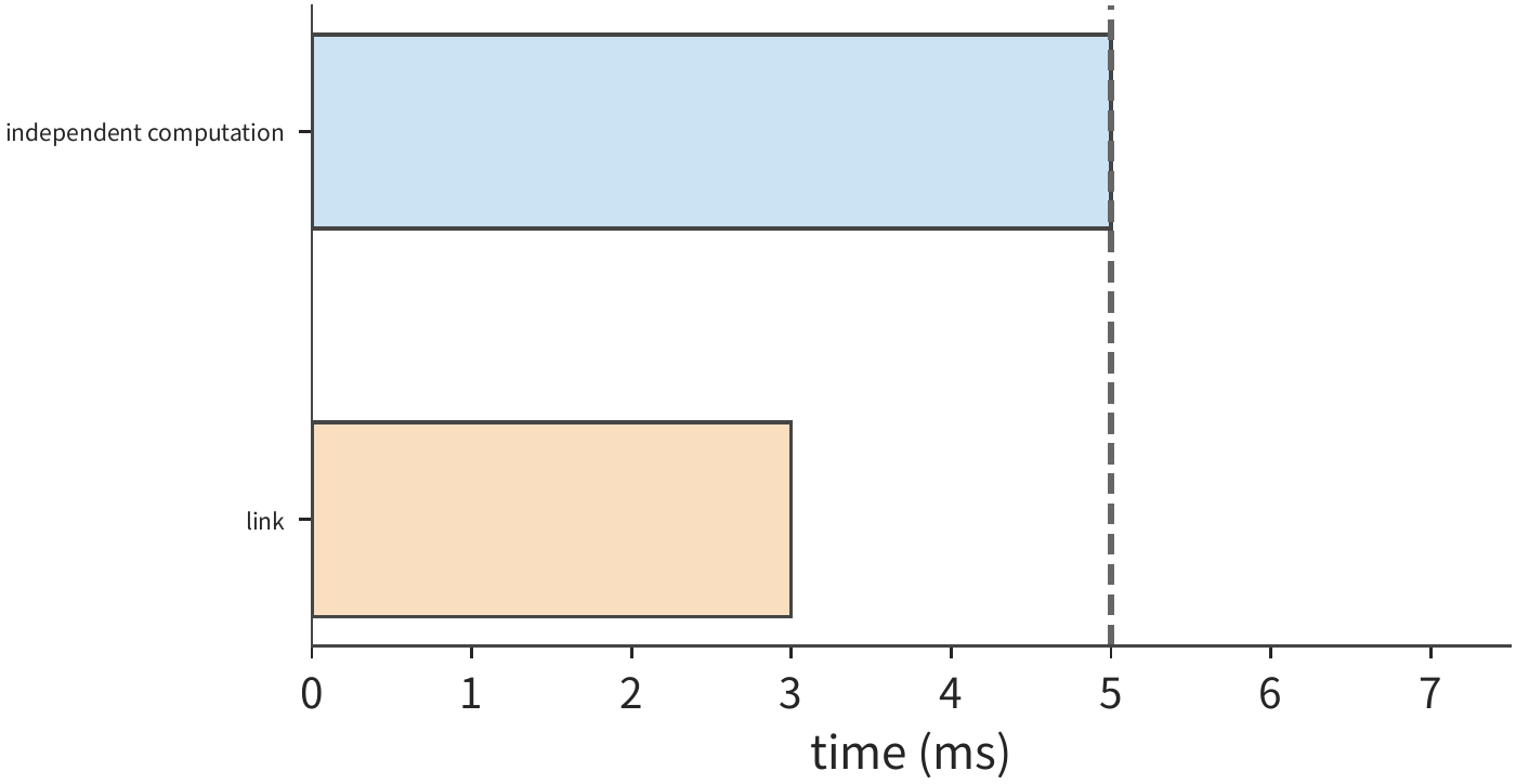
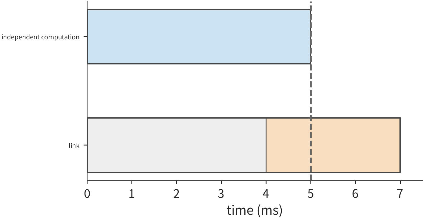
Figure 10-25 temporarily fixes the moment at which the gradient is produced. In actual training, the computation order can also be changed so that certain gradients are produced earlier, thereby moving the reduction earlier on the timeline. In matrix backward computation, the input gradient \(dX\) is passed to the previous layer to continue backpropagation, while the parameter gradient \(dW\) is handed to this layer's reduction. Computing \(dX\) first lets the previous layer start backpropagation earlier; computing \(dW\) first lets this layer's gradient communication start earlier. When the two compete for the same compute resource, changing the order reallocates the communication window. This is also why training scheduling must account for both forward and backward dependencies simultaneously.

Now use this rule to compute the communication wait time for the design case. Both schemes use full-group ZeRO-3; each micro-batch requires three collective communications: an AllGather to collect BF16 weights before the forward pass, another AllGather before the backward pass, and a ReduceScatter on the BF16 gradients after the backward pass. In each collective communication, the bytes each card sends and receives are \((d-1)/d\times2N\), about 16.0 GB at 48 cards. Each card accumulates \(m\) micro-batches, and the communication volume for one step is

\[ V=3m\cdot\frac{d-1}{d}\cdot2N. \]

At 48 cards, \(m=8\), \(V\approx385\) GB; at 32 cards, \(m=12\), \(V\approx571\) GB. The transmission path for these bytes is determined by the hardware. The RTX 4090 has no NVLink and does not support cross-card P2P (one card directly reading/writing another card's GPU memory over PCIe); even two cards in the same host must exchange data through host memory, so every send and receive on each card must pass through its own PCIe 4.0 x16, 32 GB/s per direction. Based on a published 4090 cluster configuration, each eight-card host is equipped with eight 200 Gbit/s NICs, 25 GB/s each; ring collective communication spreads cross-host traffic across the eight NICs, so the NICs are not the bottleneck. The link time per step at 48 cards is thus about \(385/32\approx12.0\) s, and about 17.9 s at 32 cards.

Link time is not the same as communication wait time. ZeRO-3 prefetches a layer's parameters before executing that layer, and reduces its gradients immediately after that layer's backward pass finishes. At 48 cards, the link time per micro-batch is about 1.50 s, while the computation for that micro-batch is about 6.53 s; layer by layer, collecting one layer's roughly 0.39 GB of parameters takes only about 12 ms, also far shorter than that layer's computation. So most communication can fit within the computation. MegaScale takes the same approach in data parallelism, and notes that the only communication that cannot be hidden is the first AllGather and the last ReduceScatter within a step. For Qwen3-8B, both of these communications act on the roughly 1.24 GB word embedding: the word embedding is the first layer in the forward pass and also the last layer whose gradient is computed in the backward pass. The two together total about 0.08 s, which is the communication wait time per step. Parameter updates and non-matrix operations within a card are already included in the per-card compute efficiency; the per-step times for the two schemes when input is ready are about 78.4 s and 52.3 s, respectively.²⁷

Most communication is covered by computation, and this also sets an upper bound on optimization gains. If only 0.2 s of a 1.3 s reduction extends past the end of backward computation, and everything else on the timeline stays fixed, then eliminating this communication wait shortens the step by at most 0.2 s. If the target still requires shortening by 0.5 s, other work on the critical path must also be shortened simultaneously.

Case: with global batch size fixed, how much speedup does a fourfold increase in card count give? The large-scale distributed training system MegaScale kept the global batch size at 6144 for a 175B model while increasing the card count from 3072 to 12288. The original per-step time was about 23.7 s; if a fourfold increase in card count gave a fourfold speedup, the per-step time should shorten to about 5.9 s, but the actual result was about 6.3 s. The overall speedup is about 3.7x, corresponding to about 93% scaling efficiency. As the card count increases, the work per card decreases, and the proportion of per-step time occupied by waiting caused by cross-group synchronization and load imbalance rises correspondingly; the actual per-step time exceeds the ideal by about 0.4 s, and this is the extra time that needs further analysis after scaling. Following the order in Section 1.3.4, first fold cross-group synchronization and load imbalance into the model: the more cards there are, the greater the fraction of the step spent waiting for the slowest group, and this is work inherent to scaling itself; only the remaining gap that this still cannot explain should be attributed to implementation overhead.¹²

10.3.4 Scheduling Changes for MoE and Long Context

Every forward pass of a dense model uses the full feedforward weights of each layer, so the work division under data parallelism is fairly regular. MoE routing causes different cards to receive different numbers of tokens, and varying sequence lengths also mean that the same token count corresponds to different amounts of computation. Analyzing per-step time therefore requires looking at how work is distributed across cards, and which card finishes last.

How uneven expert dispatch extends the compute time of the busiest card. Suppose the experts on two cards receive 96 and 32 token dispatches respectively, where each dispatch sends one token's feature vector to an expert, occupying one row in that expert's input matrix. Assume each dispatch takes approximately the same computation time. With 128 dispatches total, corresponding to 128 effective rows, the average per card is 64 rows, but the completion time is determined by the side with 96 rows. Adjusting the allocation to 64, 64 rows reduces the expert compute time from what 96 rows require down to what 64 rows require, a reduction of one third.

The load-balancing mechanism during training determines how samples choose experts; expert replicas and topology mapping then determine where these choices are executed.

The adjustment above assumes tokens can be freely moved between experts. The actual dispatch is determined by router scoring; the balancing mechanism can only influence the distribution of dispatches, and execution still needs an explicit rule for handling imbalance. The capacity factor \(c\) provides this rule: each expert's input matrix has at most

\[ \text{capacity per expert}=\left\lfloor c\times\frac{\text{token count}\times k}{E}\right\rfloor \]

rows, i.e., \(c\) times the average dispatch volume, where \(k\) is the number of experts each token selects and \(E\) is the number of experts. Dispatches exceeding capacity are dropped: that layer does not process those tokens, and their representations pass directly to the next layer via the residual connection; slots not filled to capacity are padded with zeros, and these rows still consume computation and communication.⁴

Substituting the earlier example: 128 dispatches, \(E=2\), \(k=1\), average 64 rows per expert. At \(c\) values of 1.0, 1.25, 1.5, 2.0, the capacity per expert is 64, 80, 96, 128 rows; the expert receiving 96 dispatches drops 32, 16, 0, 0 tokens respectively, and the two experts together pad 32, 48, 64, 128 rows with zeros. At \(c=1.0\), the total executed volume exactly equals the 128 effective dispatches, yet a quarter of them are dropped; from \(c=1.5\) onward nothing is dropped, at the cost of one third of the executed rows being zero-padding.

Now consider the routing scale of a real model. Qwen3-235B-A22B has \(E=128\) experts, and each token selects \(k=8\); 8,192 tokens produce 65,536 dispatches total, averaging 512 rows per expert. Suppose half the experts receive 1.5 times the average dispatch volume, the same 3:1 imbalance as the earlier example, with hot experts at 768 rows each and cold experts at 256 rows each. At \(c\) values of 1.0, 1.25, 1.5, 2.0, the capacity per expert is 512, 640, 768, 1,024 rows; hot experts drop 256, 128, 0, 0 dispatches respectively, together accounting for 25%, 12.5%, 0, 0 of total dispatches; zero-padded rows account for 25%, 30%, 33%, 50% of all executed rows.

Capacity factor \(c\)	Capacity per expert / rows	Fraction of dispatches dropped	Zero-padded rows as fraction of executed volume
1.0	512	25%	25%
1.25	640	12.5%	30%
1.5	768	0	33%
2.0	1,024	0	50%

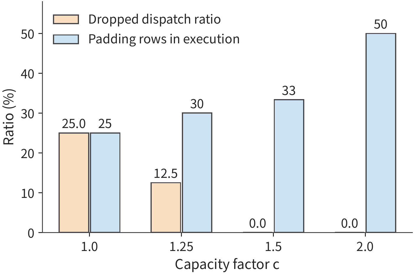
The crossover condition is determined by the routing distribution: the distribution above needs \(c=1.5\) to bring the drop rate to zero; the more balanced the routing, the closer to 1 the required \(c\), and the less zero-padding waste. The auxiliary loss (a load-balancing term added to the training objective) directly penalizes uneven dispatch; DeepSeek-V3's auxiliary-loss-free scheme dynamically adjusts routing bias based on expert load. Both push the distribution toward balance, allowing the capacity factor to take smaller values. The expert capacity formula in Section 2.4 assumes that no token dispatch is dropped during routing (\(\sum_e t_e=mk_{\mathrm{top}}\)), which corresponds to the case where the capacity factor is large enough that the drop rate is zero.⁴

Even after balancing expert computation, data transfer can still leave cards waiting. MoE's forward token exchange, backward input-gradient transfer, and parameter-gradient reduction all compete for the same link, so the communication timeline analysis from the previous section still applies. Take a 72 MiB FP32 expert gradient, reduced via ring AllReduce by the four data-parallel members holding that expert; each card sends \(2\times3/4\times72=108\) MiB. Each card is equipped with one 200 Gbit/s NIC, 25 GB/s per direction, and each collective call has a launch overhead of about 0.02 ms. The whole bucket takes about 4.55 ms, which cannot complete within a single 2 ms idle window. If the gradient is split into three 24 MiB sub-buckets, each bucket sends 36 MiB, about 1.53 ms, which can each complete within one such idle window; the total communication processing time, however, increases to about 4.59 ms. Although two more communications are launched, each small bucket finishes transmitting before computation ends, thereby reducing the wait after computation. Switching to a 400 Gbit/s NIC, the whole bucket takes about 2.28 ms, still unable to fit into the 2 ms gap, so splitting the bucket remains necessary.¹³

Expert load depends on how many token dispatches each card's experts receive. Long context introduces another kind of difference: even with the same total token count, the number of attention pairs to compute can differ.

With the same total token count, how uneven sequence lengths increase attention computation. For a causal sequence of length \(s\), the first token attends to one token, the second to two, and so on, giving \(s(s+1)/2\) effective attention pairs. Two sequences of length 4096 and 4096 together yield about 16.8 million pairs; changing to 7168 and 1024, with the total token count still 8192, increases the pair count to about 26.2 million, an increase of about 56%. The number of attention pairs grows roughly quadratically with sequence length, so longer sequences increase the total computation.¹⁴

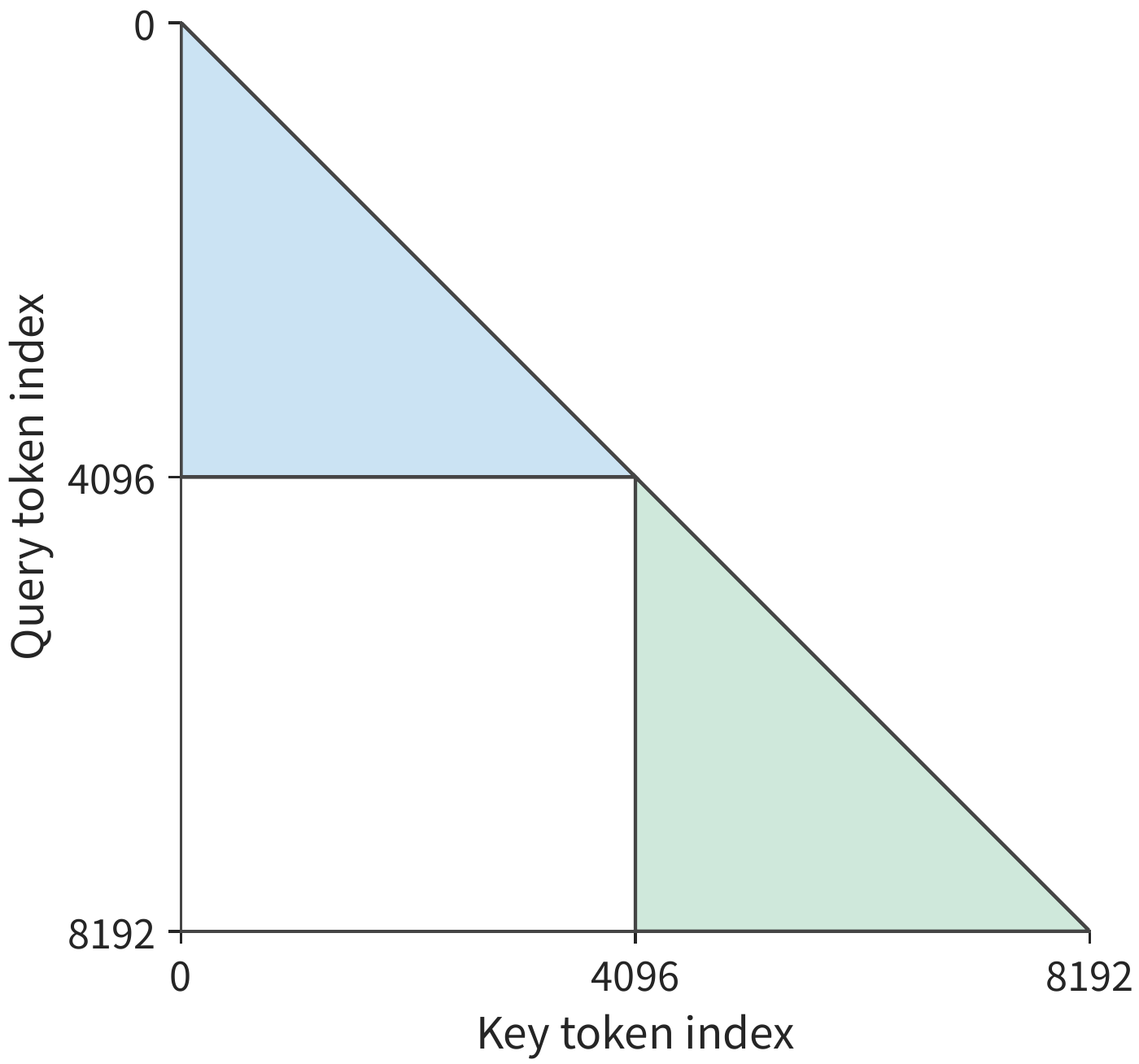
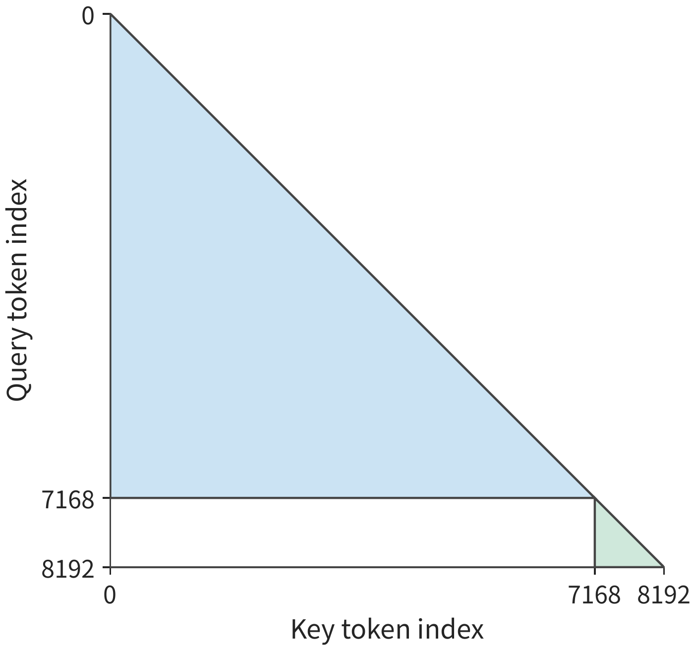
In Figure 10-29, the extra area of the longer triangle comes from genuine attention relationships and cannot be eliminated by removing padding tokens. Packing (concatenating several shorter sequences end to end into one sequence of the target length) reduces padding tokens, while length-based grouping brings the triangular area handled by each card closer together; context parallelism further splits the computation of long sequences across multiple cards, exchanging K and V held by other cards. The three approaches change, respectively, wasted work, work allocation, and the data arrival path. When comparing schemes with the same total token count, keeping the length distribution, the visibility mask (which specifies which context tokens each token position can read), and the loss weights unchanged separates the scheduling gain from changes in the task itself.

10.4 Data Input, Checkpointing, and Failure Recovery

The per-step time analysis in Section 10.3 assumed the input data was already prepared and that training was not interrupted by failure. During sustained operation, data reading and preprocessing must keep up with the pace of computation, and there must also be checkpoints saving recoverable training state. This section adds both factors to the completion time introduced at the start of the chapter: input determines whether cards can keep working continuously, and recovery determines how much of the already-completed work must be redone.

10.4.1 Data Reading, Packing, and Prefetching

Raw data goes through reading, decoding or tokenization, and filtering, is then concatenated into training sequences of the target length, placed into a host memory buffer, and finally transferred to the GPU. The host buffer typically uses pinned memory, keeping the data resident in physical memory during asynchronous transfer. The sustained processing speed of each stage determines the input speed, and queues buffer short-term speed fluctuations.

That the GPU ultimately receives a small volume of data does not mean the preparation process before it is equally fast. A 25-day budget requires about 46,300 tokens/s, i.e., about 5.7 sequences of 8,192 tokens per second. If token IDs are transmitted as int64, 8 bytes per ID, the data rate is only about 0.37 MB/s. Suppose each CPU data-preparation process prepares two sequences per second; two data-preparation processes yield only four sequences/s, below the requirement; three data-preparation processes reach six sequences/s. Even though the transferred data volume is small, the preparation process on the CPU can still slow down the whole cluster.

The design case in this chapter allocates four such data-preparation processes for input, totaling eight sequences/s. At 48 cards, the per-step time with input ready is about 52.3 s, processing 384 sequences per step, requiring about 7.3 sequences/s, below eight sequences/s. Data preparation runs faster than training consumes, so after a brief slowdown the prefetch queue can be refilled. The design case further allows 0.5 s of average input wait per step to represent the wait that prefetching fails to eliminate, changing the per-step training time at 32 and 48 cards to about 78.9 s and 52.8 s.²⁷

The prefetch queue lets data preparation and GPU computation run at different paces. During normal training, data prepared in advance can relieve the wait caused by fluctuations in input speed; when saving a checkpoint, however, it is essential to distinguish which data has already been used for training. Suppose the data loader has already assigned preparation tasks for the first 108 batches, while training has completed only batch 100; batches 101–108 are still being processed or queued. If recovery resumes directly from batch 109, eight batches would be skipped. The batch position already assigned to the data-preparation processes reflects prefetch progress, while the batch position already used in training reflects training progress; the buffer between the two holds data not yet trained on.

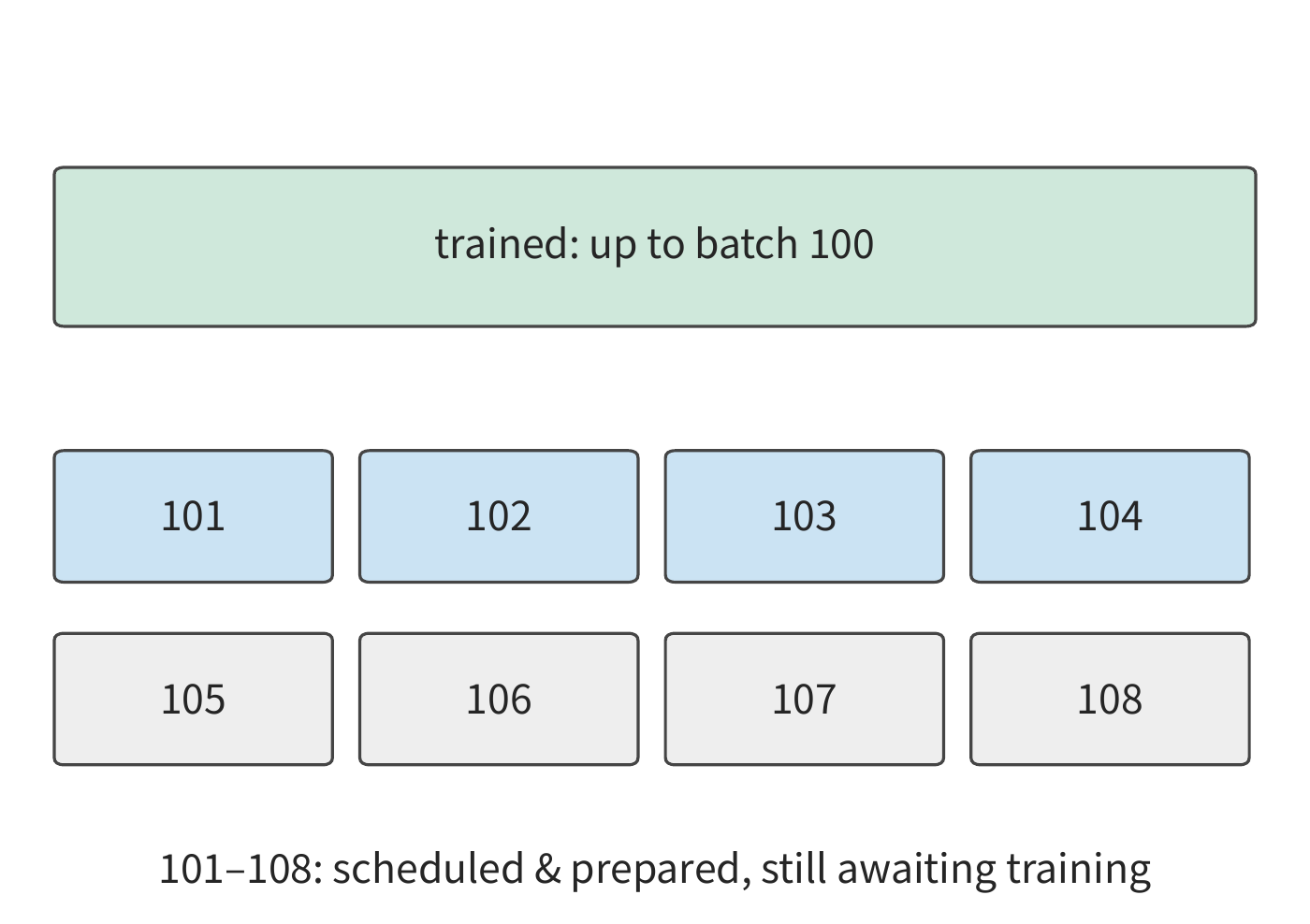
The queue in Figure 10-30 can only temporarily compensate for a slowdown in preparation speed; if data preparation remains slower for a long time, the queue will eventually be drained. Checkpoint writing is subject to the same constraint: once the average rate at which snapshots are produced exceeds the rate storage can sustainably accept, the backlog of pending writes keeps growing, and the finite staging buffer will eventually be filled; Section 10.4.4 computes this kind of backlog using specific write rates. For the text task in this chapter, the input side involves a small byte volume, with the bottleneck in CPU-side data preparation; the average write traffic for checkpoints is also not large: the design case uses an 1800 s save interval, and the roughly 115 GB checkpoint averages only about 64 MB/s. The stall caused by saving is accounted for separately in Section 10.4.4.¹⁵

10.4.2 Recoverable State and Layout Transformation

Suppose training just completed a parameter update, and the machine stops at that point. To resume training after recovery, one needs to know the weights at that time, which batch of data to read next, and what history the optimizer has already accumulated. Weights alone are enough to run forward inference, but not enough to determine the next training update. A training checkpoint must therefore save all the necessary state corresponding to the same point in training, so that training can continue after recovery.

Training with Adam, as used in this chapter, requires saving the weights, the first and second moments, the step count, the learning rate state, the random state, and the composition of the next batch of data. The learning rate controls the update step size, and the random state determines the sequence of subsequent random sampling. With the same weights but different optimizer moment states, the next parameter update may differ; with the same data reading position but different leftover tokens from packing, the next training sequence will also change. What the activation recomputation in Section 10.2.2 addresses is which intermediate values within a single forward-backward pass can be reconstructed; what a checkpoint must address is how the entire training process continues after an interruption.

After one training iteration ends, the next batch of gradients is regenerated by the backward pass. At this point, the saved state consists of weights at 2 bytes, master weights at 4 bytes, and two Adam states at 8 bytes, totaling 14 bytes per parameter. This portion of the Qwen3-8B checkpoint is about 115 GB. Saving the model state together with the data position already processed, at the end of a training iteration, determines which parameters to use after recovery and from which batch to continue training.

Recovery may also require changing the parallelism layout, requiring the same state to be resharded. Example: how is a checkpoint resharded from four-way tensor parallelism to eight-way? The gate projection weight has shape \([12288,4096]\), 96 MiB in BF16. Split fourfold along the output dimension, each shard has 3072 rows, 24 MiB; split eightfold, each shard has 1536 rows, 12 MiB. The target card with rank \(r\) reads the old shard \(\lfloor r/2\rfloor\), with even ranks taking the first half and odd ranks the second half. Global row coordinates connect the old and new layouts.

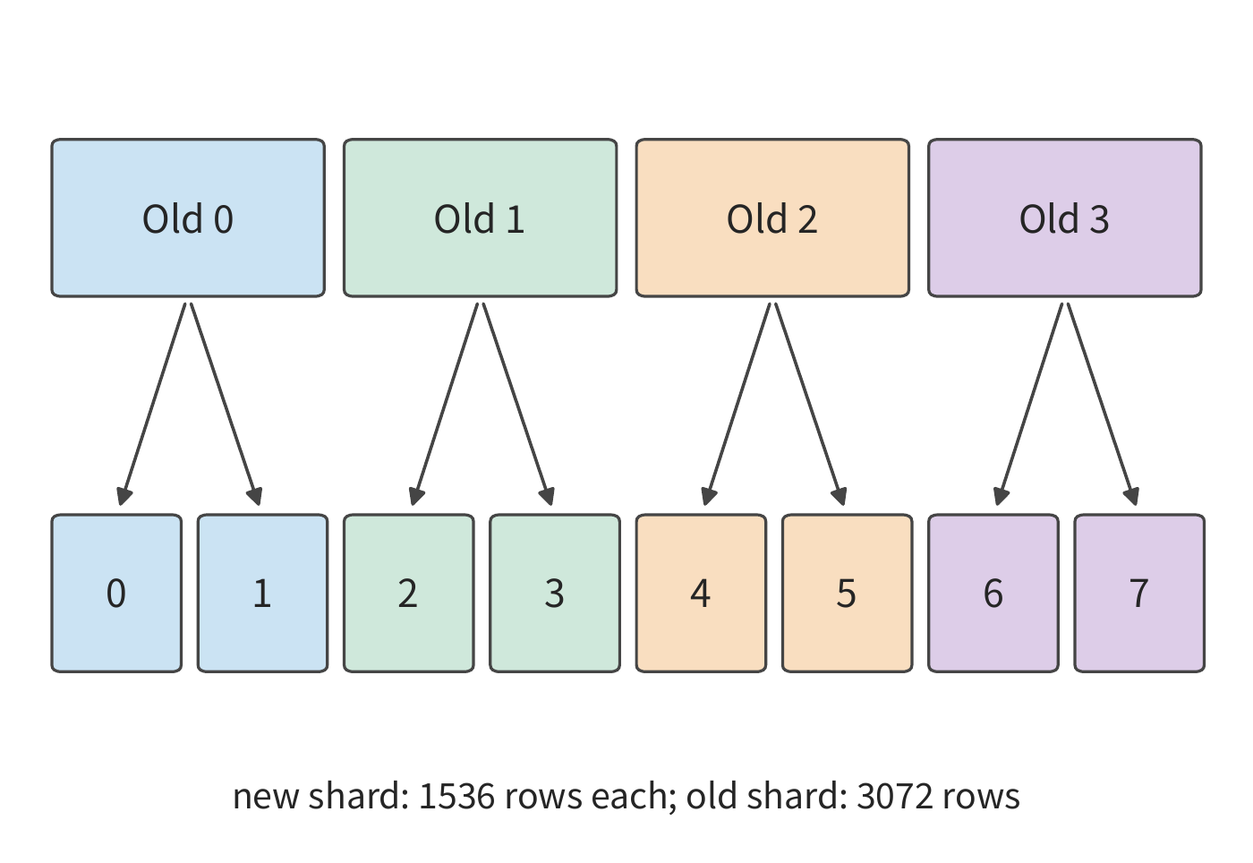
Following the arrows in Figure 10-31, the recovery program can find the original row range corresponding to each new shard. The FP32 master weights and the two Adam states are also split along the same row ranges, each twice the size of the BF16 weights. The total state for this matrix in the checkpoint is therefore \(96\times(1+2+2+2)=672\) MiB. Systems such as ByteCheckpoint describe these tensors using global shape, offset, and shard length, letting the recovery program read the needed range according to the target layout. File sharding is a storage arrangement, while global coordinates indicate which tensor a shard belongs to and which rows and columns it occupies.¹⁶

Weights can be reassembled using the original matrix's row numbers, but training sequences also need enough retained information to reconstruct the same input. The data in Figure 10-30 that is already prepared but not yet used in training likewise needs to be relocated correctly at recovery time. Besides the batch position, the intermediate results of data preprocessing must also be retained.

If the packer retains 2,000 tokens, and the next batch of data provides 6,192, the two together form the next 8,192-token sequence. If these 2,000 tokens were lost, extra tokens would have to be drawn from subsequent data to fill out the next sequence, thereby changing its prefix, attention relationships, and labels. Saving the data position already used for training, the tokens not yet forming a complete sequence, and the parameter update result together allows the same batch of data to be reconstructed after recovery.¹⁷

10.4.3 Synchronous Saving, Asynchronous Saving, and Bandwidth Contention

This section discusses how the saving process proceeds alongside training, and when a snapshot actually becomes usable.

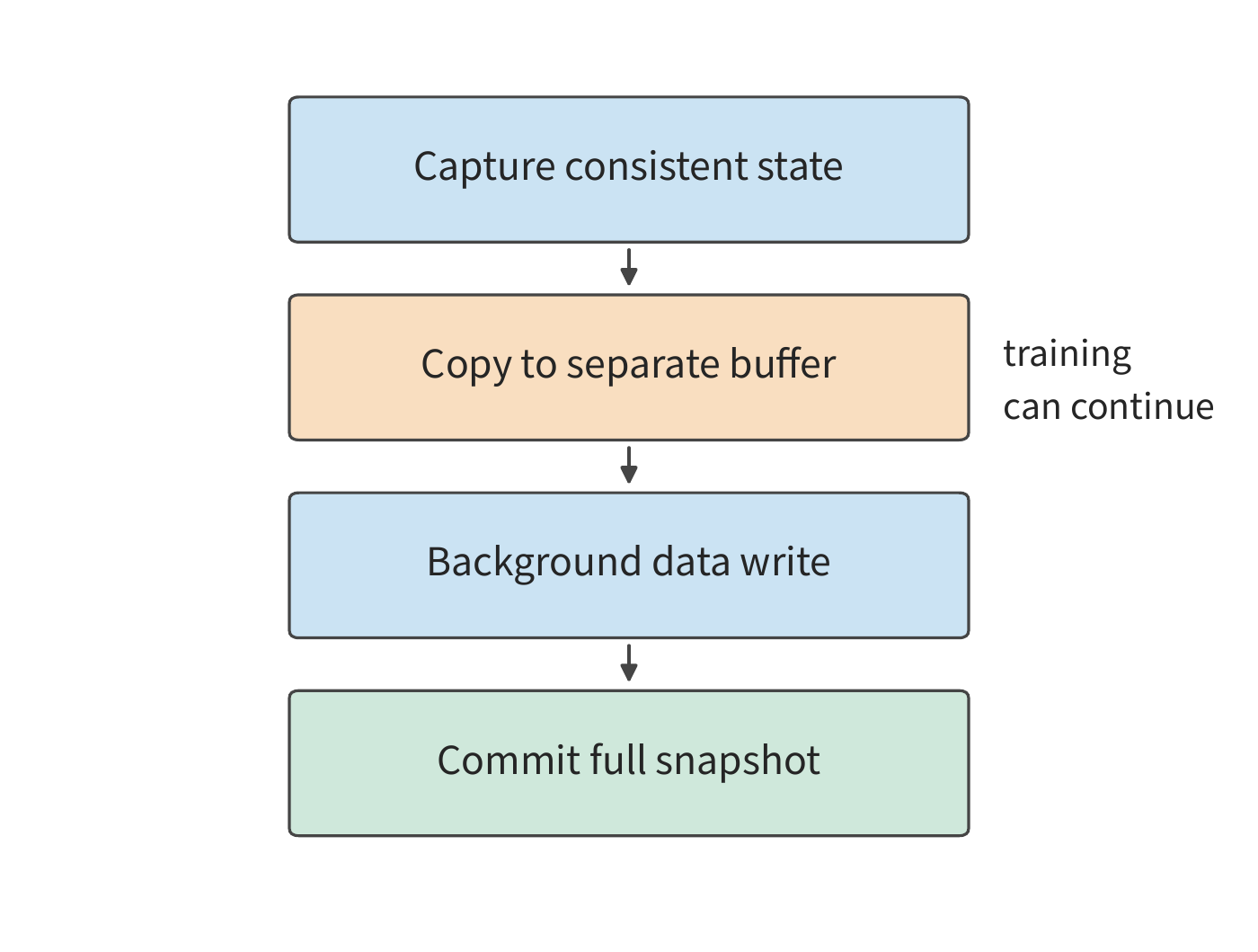
Synchronous saving first produces a snapshot with fixed content, and training continues only after the write completes. Asynchronous saving copies the snapshot to an independent memory buffer, then has a background process write it out, letting training resume execution sooner. When training resumes execution, the snapshot may not yet be fully written; only once the write is complete and committed can this snapshot be used for failure recovery.

Example: how does checkpoint upload speed determine the amount of rework after a failure? Take a snapshot of 112 GB each. The DGX SuperPOD reference architecture gives storage performance tiers by workload; NLP training corresponds to the Good tier, where one SU (a scalable unit made of 32 DGX systems) has a combined storage write throughput of 7 GB/s; at this rate, writing one snapshot takes 16 s. Producing one snapshot every 10 s gives a data production rate of 11.2 GB/s, and the queue keeps growing. Changing to one snapshot every 20 s lowers the average demand to 5.6 GB/s, letting storage finish writing the previous snapshot before the next one arrives.

Capturing two snapshots at the 20th and 40th seconds, each takes 0.5 s to copy to the buffer before uploading, completing at 36.5 and 56.5 s. If a failure occurs at the 50th second, the second snapshot is still uploading, so recovery can only go back to the 20th second, redoing 30 s. Switching to the Better tier's combined 20 GB/s write throughput, each snapshot takes only 5.6 s, completing at 26.1 and 46.1 s respectively; the same failure can recover to the 40th second, redoing only 10 s.

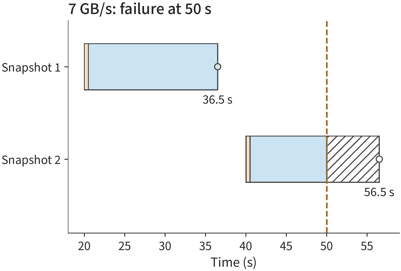
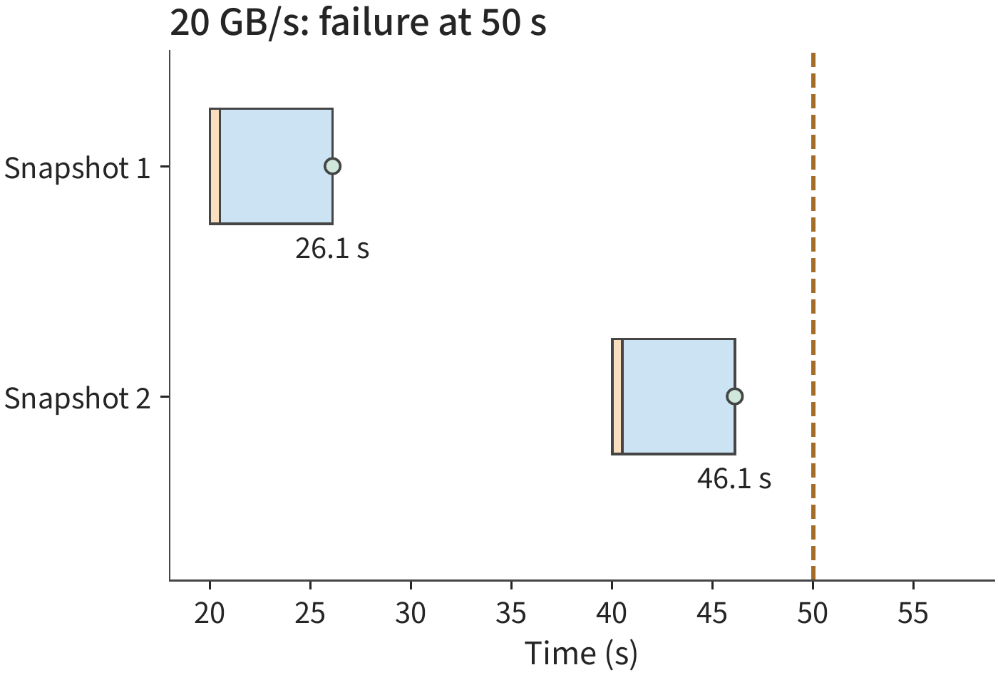
Both schemes have the same foreground pause: two pauses of 0.5 s each, totaling 1 s. Faster writing lets recovery reach a training state closer to the failure, redoing 20 s less. The asynchronous save's commit point thus directly affects long-term progress: background write speed affects the amount of rework after a failure, while the pause duration during saving extends normal running time.

Beyond writing the data files, real systems also need to commit metadata describing the complete snapshot. In one set of CPU experiments, the save API call returns in about 7 ms, while the recovery metadata takes about 48 ms to commit; if the process terminates before the commit, the recovery program selects the last complete checkpoint. The data files and the commit record together constitute a usable snapshot, and the recovery program uses this to determine which checkpoint has already been saved in full.¹⁸

10.4.4 Failure Scope, Save Period, and Effective Training Progress

Figure 10-33 fixed the timing of two saves and compared the effect of write speed. The save interval can also be changed: a short interval keeps the failure closer to the last snapshot; a long interval means fewer pauses for saving during normal training. These two costs move in opposite directions, so a trade-off point exists.

Let \(c\) be the time each synchronous save takes, \(\tau\) the seconds of useful training completed between saves, \(\lambda\) the job's failure rate, and \(r\) the recovery time. Assuming failures occur infrequently and independently, the first-order model gives the additional cost per unit of useful training time as

\[ L(\tau)=\frac{c}{\tau}+\lambda\frac{\tau}{2}+\lambda r. \]

The first term comes from saving once every \(\tau\) seconds. A failure can land at any point between two saves, losing half the interval on average, which gives the second term. The third term is the expected number of recoveries per unit of useful training time multiplied by the recovery time per event. The first two terms decrease and increase respectively, and the optimum satisfies

\[ -\frac{c}{\tau^2}+\frac{\lambda}{2}=0, \qquad \tau^*=\sqrt{\frac{2c}{\lambda}}. \]

Example: how do card count and failure rate determine the checkpoint save interval? Meta's statistics on a research cluster's training jobs show that a 1024-card job is interrupted on average once every 7.9 hours, and the interruption rate is proportional to card count, equivalent to roughly one failure per card every 337 days. Any single card failure interrupts the whole job. A roughly 115 GB checkpoint saved at 7 GB/s gives \(c\approx16.4\) s. Assuming recovery takes 120 s, substituting gives an optimal interval of about 965 s, or roughly 16 minutes.¹⁹

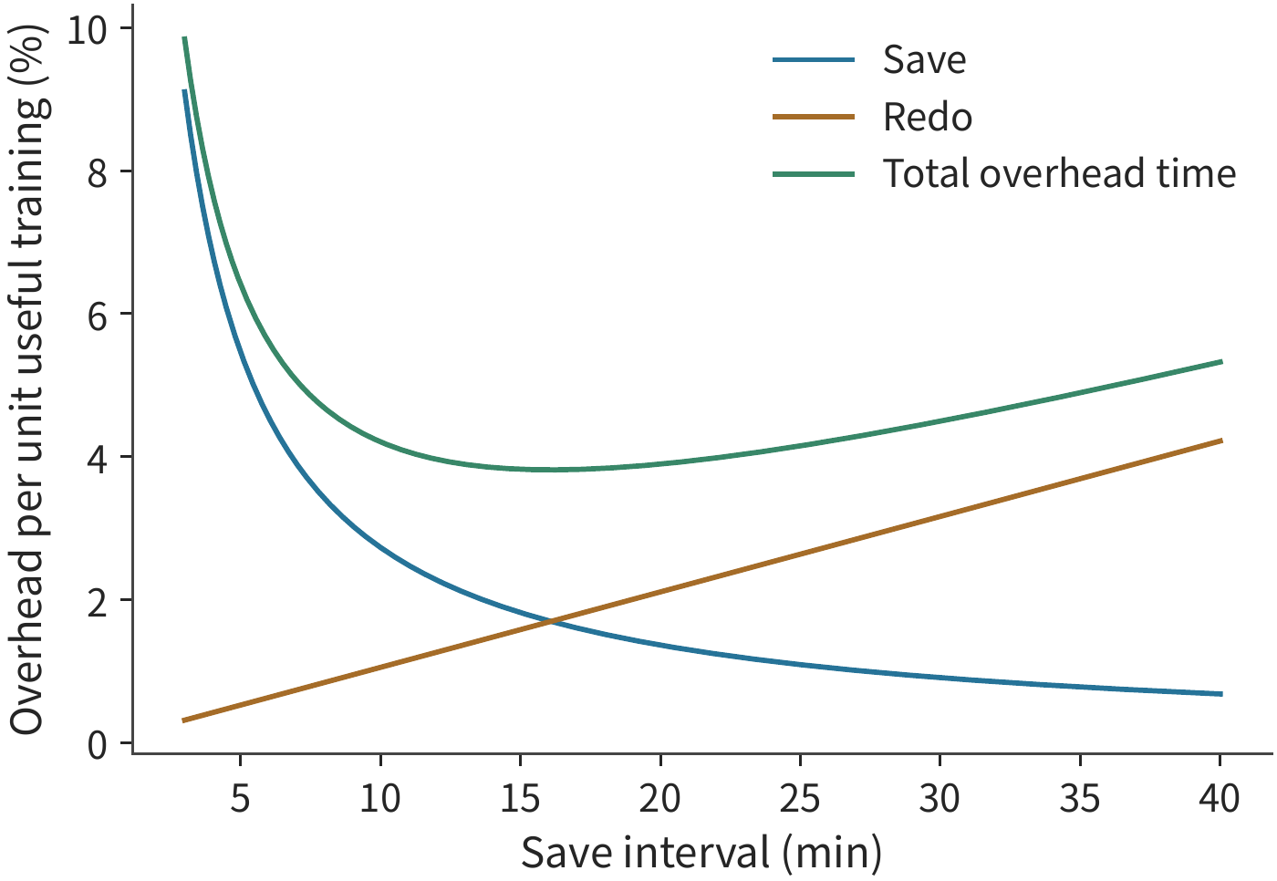
The minimum in Figure 10-35 is fairly flat, so a convenient nearby interval can be chosen in configuration. The table below compares five, fifteen, and thirty minutes, showing which cost increases as the interval moves away from the minimum.

Useful training interval	Save cost	Rework cost	Recovery cost	Total
300 s	5.5%	0.5%	0.4%	6.4%
900 s	1.8%	1.6%	0.4%	3.8%
1800 s	0.9%	3.2%	0.4%	4.5%

Extending the save interval from five minutes to fifteen minutes saves more save time than it adds in rework time; extending further to thirty minutes, the added rework time exceeds the save time saved. The totals in the table are computed from unrounded values. Doubling card count doubles the failure rate, shortening the optimal interval to \(1/\sqrt2\) of its original value; doubling save speed shortens the optimal interval by the same factor, since each save takes less time.

The design case in this chapter uses fewer cards, following the assumption of roughly one failure per card every 337 days (mean time between failures per card, MTBF), a 120 s recovery time, and a roughly 16.4 s save time, taking a useful training interval of 1800 s. For 32 cards, the combined save, rework, and recovery cost adds about 1.02% of time; for 48 cards, about 1.08%. The 48-card scheme has a higher probability of being interrupted by a card failure, but the added fraction is only about 0.06 percentage points more, far smaller than the benefit gained from shortening single-card computation time. Capacity, per-step training time, and long-term added cost are now all in place; Section 10.6 will aggregate them into completion time.

At large training scales, even an interruption lasting only two or three hours can consume tens of thousands of dollars in resources. The checkpoint interval determines how much work must be repeated after a failure; system reliability determines how often that loss occurs.

Example: how much money does a training interruption waste? Xiaomi's MiMo-V2.6 was the first frontier-lab project to livestream its RL training process. The public dashboard reported RL post-training costs of roughly $2.6 million for Pro and $0.9 million for Flash, the two model sizes, at approximately $20,600 and $10,300 per hour, respectively.

Figure 10-36 plots the two runs from their logs. Pro restarted 14 times. Its interruption intervals totaled about 30.1 h (23.6% of total runtime), corresponding to approximately $619,000. Before Pro's fifth restart, 2.76 h had elapsed since the previous step completed, costing about $56,700; the sixth and eighth intervals lasted 2.63 h and 2.95 h, corresponding to about $54,100 and $60,700. The restarts had three main types of cause: hardware faults such as GPU-memory double-bit errors; service failures such as container crashes and loss of network access to the grader; and memory exhaustion, including exhausted KV caches during inference, GPU out-of-memory errors caused by expert-load imbalance during training, and host-memory exhaustion during sequence packing. In Flash, an infrastructure error went undetected until after step 17 had completed, forcing training to restart from step 15. The roughly four hours already spent on steps 16 and 17 were consequently wasted.⁵

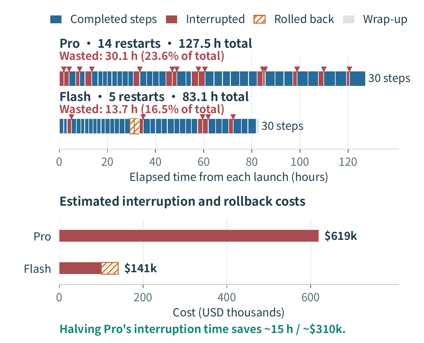
If Pro's total interruption time were halved, the same training work would take about 15 fewer hours, saving roughly $310,000 at the stated rate. There are two ways to achieve this. One is to eliminate recurring faults: the MiMo team, for example, adjusted training parallelism to reduce activation memory and accommodate peaks in expert load. The other is to detect failures earlier, recover faster, and use a more recent checkpoint to reduce rework, shortening recovery time \(r\) or the interval of training progress lost.

10.4.5 Stragglers and Slow Nodes

The model in the previous section treats failure as an event that interrupts the job. There is also a more frequent kind of degradation that does not interrupt the job: a card computes slowly on a given step. In synchronous data parallelism, each step must wait for the slowest card to finish; the card that slows down the whole step is called a straggler, so step time is determined by the maximum across cards rather than the mean. Let per-card computation time be i.i.d. with mean \(\mu\) and standard deviation \(\sigma\); with \(N\) cards, the computation portion of step time is the maximum of \(N\) samples. Taking \(\mu=52.2\) s (the per-card computation time of the 48-card scheme) plus 0.58 s of communication and input waiting per step, we take \(\sigma\) as 2% of the mean (1.04 s) and 5% (2.61 s) respectively.⁶

The expected maximum of \(N\) independent normal samples equals \(\mu\) plus some multiple of \(\sigma\): for \(N=8,48,1024\), the multiples are about 1.42, 2.23, and 3.25 respectively. Substituting gives the expected per-step time:

Cards	\(E[\max]-\mu\) (multiples of \(\sigma\))	Per step, \(\sigma=2\%\) / s	Per step, \(\sigma=5\%\) / s
8	1.42	54.3	56.5
48	2.23	55.1	58.6
1024	3.25	56.2	61.3

Without variation, each step takes about \(52.2+0.58\approx52.8\) s. The more cards, the larger the expected maximum: with 48 cards and \(\sigma=5\%\), each step takes about 5.8 s longer, consuming four-tenths of the roughly 14.4 s margin from Section 10.6; with 1024 cards, about 8.5 s longer. Slow cards can be detected from communication waiting: each card's wait time on the gradient bucket AllReduce equals the step's end time minus its own computation end time; for a card whose computation time is exactly the mean, the expectation of this wait is precisely \(E[\max]-\mu\).⁶

Once a slow card is detected, there are three responses: waiting, reallocation, and eviction. Waiting: the current step ends according to the slow card's time. How much extra time a card slowed to \(\mu+3\sigma\) makes the rest wait depends on how large the maximum of the remaining \(N-1\) cards would already be: at \(\sigma=2\%\), 8 cards wait an extra ~\(1.65\sigma\) (1.72 s), 48 cards wait an extra ~\(0.78\sigma\) (0.81 s), and at 1024 cards the maximum of the remaining cards already exceeds \(\mu+3\sigma\), so the extra wait is zero. Reallocation: the slow card's work is spread evenly across the remaining \(N-1\) cards, making the mean \(\mu N/(N-1)\). Still taking \(\sigma=2\%\) and ignoring migration cost, 48 cards give about 56.2 s per step, and 8 cards rise to about 61.6 s, both higher than the expected step time under waiting at the same \(\sigma\) (55.1 s and 54.3 s): spreading the load makes each card do \(1/(N-1)\) more work, and this increment exceeds the wait caused by one slow card, with the gap larger when there are fewer cards. Eviction: the slow card is removed from the job, and the job restarts from the last checkpoint, at a cost of expected lost work \(\tau/2\) plus recovery time \(r\). Taking a save interval shorter than the design case's 1800 s, \(\tau=600\) s, with \(r=120\) s, gives a cost of 420 s, roughly eight steps at 52.8 s per step under the 48-card scheme. A single \(\mu+3\sigma\) jitter only costs a few seconds, so eviction is only worthwhile when a card stays slow for many steps. Real clusters do have slow cards: MegaScale reports about 0.5% of machines are noticeably slower; the Meta cluster statistics in Section 10.4.4 give the relationship between job scale and interruption — a 1024-card job has a mean time between failures of 7.9 hours, while an 8-card job has 47.7 days.⁶

Besides hardware failures, there is another kind of event requiring a checkpoint rollback: the loss spike from Section 10.1.2. A loss spike does not damage hardware, but is handled the same way — discarding the current parameters and returning to the last snapshot — and it affects the save period the same way as a hardware failure. Treating loss-spike-induced rollback as a shock affecting the entire job simultaneously, occurring on average once every \(1/\lambda_{\mathrm{spike}}\), the first-order model from the previous section is corrected to

\[ L(\tau)=\frac{c}{\tau}+(\lambda_{\mathrm{hw}}+\lambda_{\mathrm{spike}})\left(\frac{\tau}{2}+r\right), \qquad \tau^*=\sqrt{\frac{2c}{\lambda_{\mathrm{hw}}+\lambda_{\mathrm{spike}}}}. \]

Using the 48-card hardware failure rate (per-card MTBF of about 337 days), and assuming loss spikes cause a rollback on average once every seven days: still at \(\tau=600\) s, the added fraction rises from 2.80% to 2.87%, and the optimal save period shrinks from about 4,458 s to about 3,150 s. At the design case's 1800 s interval, the added fraction changes from 1.08% to about 1.25%, increasing completion time by about 0.03 days, which does not change the scheme choice in Section 10.6. The crossover condition is given by the relative magnitude of the two rates: the more frequent the spikes, the shorter the optimal period; when \(\lambda_{\mathrm{spike}}\gg\lambda_{\mathrm{hw}}\), the save period is determined almost entirely by numerical stability; when the rollback interval is on the order of months, it has almost no effect on the 1.08% added fraction.⁶

10.5 Reinforcement Learning Training

The previous four sections assumed the training data was already given. RL lets the model participate in producing the next batch of data: the model generates trajectories, the system computes rewards or verification results, the trajectories are then used for training, and the updated weights in turn change the next round of generation. The system changes from a training pipeline processing fixed data into a feedback loop, and new problems center on the processing speed of each stage, the state overlap during transitions, and exactly which policy version produced a given sample. The inference side generating trajectories and the training side computing loss must also give alignable probabilities for the same trajectory — this is this section's training-serving consistency. Training-serving consistency directly affects whether parameter updates follow the algorithm's expectations, and constrains the benefit of stage acceleration and asynchronous execution.

10.5.1 One Round of Response Generation, Verification, and Parameter Update

The completion process of one round of the feedback loop is as follows. Starting from four prompts, two responses are generated per question, giving eight trajectories. The reward describes the outcome of these responses, and the advantage measures how much better a response is than the chosen baseline, which is used to determine the direction and magnitude of adjusting response probability. The training side constructs the loss over the effective tokens and completes one parameter update. Once the new weights are handed to the generation side, the next round of samples comes from the updated policy. Generation, reward, and learning each use different forms of data, and sample identifiers connect all three.

The data source here differs from the fixed dataset typically used in SFT. SFT predicts the next token on a ground-truth prefix given the answer — that is, teacher forcing — but at deployment time the model continues its response based on its own generated prefix. Once an earlier generation is wrong, subsequent generation may enter contexts less covered by the training data, and error accumulates as generation proceeds. This distribution shift between the training prefix and the usage-time prefix is one limitation of fixed-data SFT. The gradient still correctly corresponds to the current loss, but the situations covered in training differ from those the model actually encounters.

To address this prefix distribution shift, OPD has the current student model generate its own trajectories, and a teacher then provides supervision for the prefixes the student actually generates, for example the next-token probability distribution. The student can thus learn at the positions where it is prone to error, reducing prefix distribution shift; the teacher's per-token feedback also provides a finer learning signal than a single terminal reward. DeepSeek V4 uses multi-teacher OPD to merge domain expert capabilities into a unified model, and Chapter 3 has already listed teacher forward passes as an independent computational workload.²²

Compared with fixed-data SFT, OPD's potential advantage is that the number of learning samples or updates needed to reach a target capability may be reduced. It simultaneously increases the cost of student online generation, teacher forward passes, and weight synchronization, and whether it reduces total GPU-hours or completion time still needs to be measured empirically. SFT describes a supervised objective, while offline describes whether the data is fixed in advance; it is also possible to collect data online and then use a supervised loss. Online means data is continuously produced as training proceeds, while on-policy further requires that the sampling distribution match the policy being optimized. Asynchronous online RL may use a lagged policy, and OPD also encounters computational differences between the generation engine and the training engine. Therefore, online sampling is used to mitigate data distribution shift, while training-serving consistency also requires aligning the computational processes on the generation and training sides.

Returning to the eight trajectories from the round at the start of this section, consider how the training side constructs the loss over effective tokens. The eight-response example from Section 10.3.1 comes from a small-model experiment's response lengths: the responses contain 20 effective tokens in total, including the EOS token marking end of sequence; the input contributes 366 effective tokens for computation. Both the prompt and the response participate in the forward computation, while the loss is normalized over the selected response tokens. Generation length therefore affects computation cost; the loss mask indicates whether each token counts toward the loss, determining which tokens participate in gradient computation. The two roles are distinct.²⁰

Beyond the loss, the relative reward within the same prompt also determines the advantage. For example, if two responses both get a reward of 1, subtracting the group mean gives zero for both; if the rewards become 1 and 0, centering gives 0.5 and −0.5, and only then does the policy get a direction for distinguishing the two responses. Even after the system completes the forward pass, backward pass, and optimizer call, it may still encounter a batch where the first kind of situation — all advantages zero — occurs. When measuring training throughput, one should count the actual number of trajectories or tokens used for training per second; whether model capability improves should be checked with fixed evaluation tasks.

Case: parameters changed, so why didn't model capability improve? In one fixed small-model experiment run with the RL training framework verl and the inference engine vLLM working together: an exact-match reward on arithmetic problems gave the same reward to responses within the same group, so the advantage and policy gradient were both zero, and the only parameter change came from AdamW's weight decay. Beyond Adam's gradient update, AdamW separately shrinks the weights by a proportional factor; even when the current policy gradient is zero, this step still changes the parameters. Switching to a fixed sign reward instead, both training steps showed nonzero gradients and weight updates, but arithmetic verification was only 2/4 correct. Reward construction determines the direction of learning; system execution is responsible for consistently applying that direction to the parameters.²⁰

10.5.2 Resource Allocation and Weight Synchronization Across Stages

Now that we understand how samples become gradients, we can discuss how many samples can be trained per second. RL's feedback stage may execute rule-based verification or a reward model (a model that scores responses), while OPD requires a teacher to provide supervision; both should allocate resources according to the actual throughput of the feedback work. Generation, verification, and learning are like three successive stages of a process: the earlier stage running faster only increases final output if the later stage can absorb it. First convert the throughput of the three stages into the same unit of work. Let \(r_g,r_v,r_l\) denote the three stages' throughputs, and let \(q\) be the proportion passing verification that meets the policy version requirement; under stable pipelined execution on independent resources, the upper bound on samples usable for training per second is

\[ r_{\mathrm{effective}}=\min\left(r_l,q\min(r_g,r_v)\right). \]

Example: among the three stages of RL generation, verification, and learning, which should be scaled up first? Generation provides 12 equal-length trajectories per second, verification processes six, and the learning stage processes eight; a quarter of verified trajectories are discarded for being too far out of policy version. Only \(6\times0.75=4.5\) trajectories per second enter learning. Doubling generation to 24/s, the verification bottleneck still limits the samples entering learning to 4.5/s; doubling verification to 12/s, the trajectories that can be sent to training reach nine per second, at which point the training side can only handle eight per second, becoming the bottleneck of the whole pipeline. Therefore, new resources should be allocated to whichever stage is currently slowest; after that stage speeds up, the bottleneck should be reassessed to see where it has shifted.

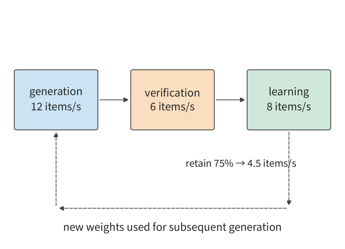
Figure 10-37 first draws the three stages on independent resources. Switching to the same group of cards running each stage in turn would reduce the number of cards needed, but generation and learning would need to switch entire sets of data in GPU memory between them.

Shared accelerators let the same group of cards alternate between training and generation, saving on duplicate resources; independent deployment lets both sides run independently, gaining overlap opportunities, but requires sending weights between two groups of cards. The key cost of shared accelerators occurs at the switch: the old state has not yet been released while the new state has already begun loading, and even though each stage individually has enough GPU memory when running alone, the switch may exceed capacity because both sets of data occupy memory at once.

Let the shared cards be H100 SXM, nominally 80 GB, about 74.5 GiB. Training state occupies 40 GiB of memory. Generation needs about 15.3 GiB of BF16 weights and a 24 GiB KV cache pool, plus 4 GiB of overhead shared by both stages. Training alone uses 44 GiB, and generation alone uses about 43.3 GiB, both under 74.5 GiB. If generation weights and KV are restored first and training state released afterward, the peak is \(40+15.3+24+4\approx83.3\) GiB, exceeding the capacity of one H100.

Changing the order — loading the weights needed for generation first, without yet allocating KV — gives a peak of \(40+15.3+4\approx59.3\) GiB. Then releasing the 40 GiB of training state drops memory usage to about 19.3 GiB, after which KV is allocated, entering the roughly 43.3 GiB generation state. Both paths reach the same final state, but the peaks differ by 24 GiB, exactly one KV pool.²¹

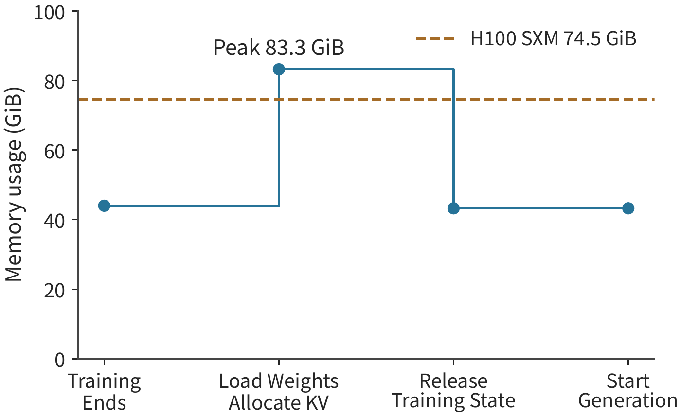
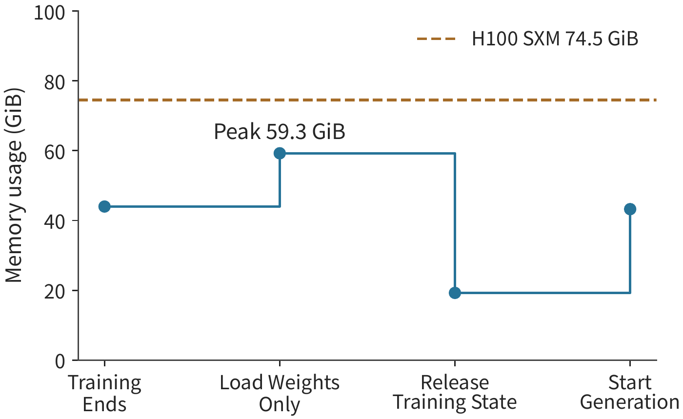
The cost of independent deployment is instead determined by the scope of weight transmission. Qwen3-235B-A22B's BF16 expert weights total 423 GiB; with 16-way expert parallelism (EP16), each receiver needs only about 26.4 GiB. Sending the complete expert set individually to 16 receivers totals \(16\times423=6768\) GiB; sending each receiver's own shard totals 423 GiB. Determining each receiver's needed parameter shard first, then organizing the distribution, can simultaneously reduce receive buffers and the sender's transmission volume.

Here, both of this chapter's analytical methods are used again: shared accelerators require analyzing tensor lifetimes, while independent deployment requires analyzing data transfer and the processing time of each stage. Once the stages are independent, differences in policy version arise; the next subsection analyzes how such version differences affect the number of samples usable for training.

There is also a category of weights with a different lifecycle in weight synchronization: the fixed-weight accelerators from Section 4.7.3 can run models in an RL pipeline whose weights remain unchanged for a long period. For example, when the algorithm uses a fixed reference model, its weights can stay in dedicated storage and be read repeatedly; the continuously updated policy model instead uses writable weight storage and publishes new versions to the generation side. Figure 10-40 draws the weight paths for these two lifecycles.

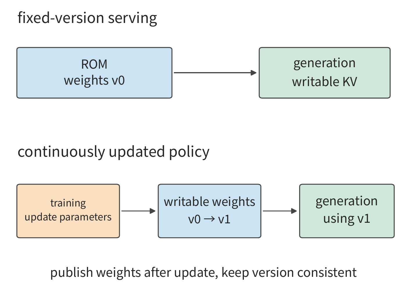
10.5.3 Asynchronous Training, Policy Version, and Long-Trajectory Recovery

The independent deployment in Section 10.5.2 further allows different batches to interleave: while the learning side is processing the previous batch of samples, the generation side has already begun generating the next batch. A synchronous loop instead waits for learning and weight synchronization to finish before producing the next batch of samples. An asynchronous loop lets generation and learning overlap, and the generation side may still be using old weights. To compute a sample's contribution to the current parameter update, the probability under the actual sampling policy must be retained.

After a weight update, the model's policy changes accordingly. Below we distinguish three policy versions along the order in which samples flow.

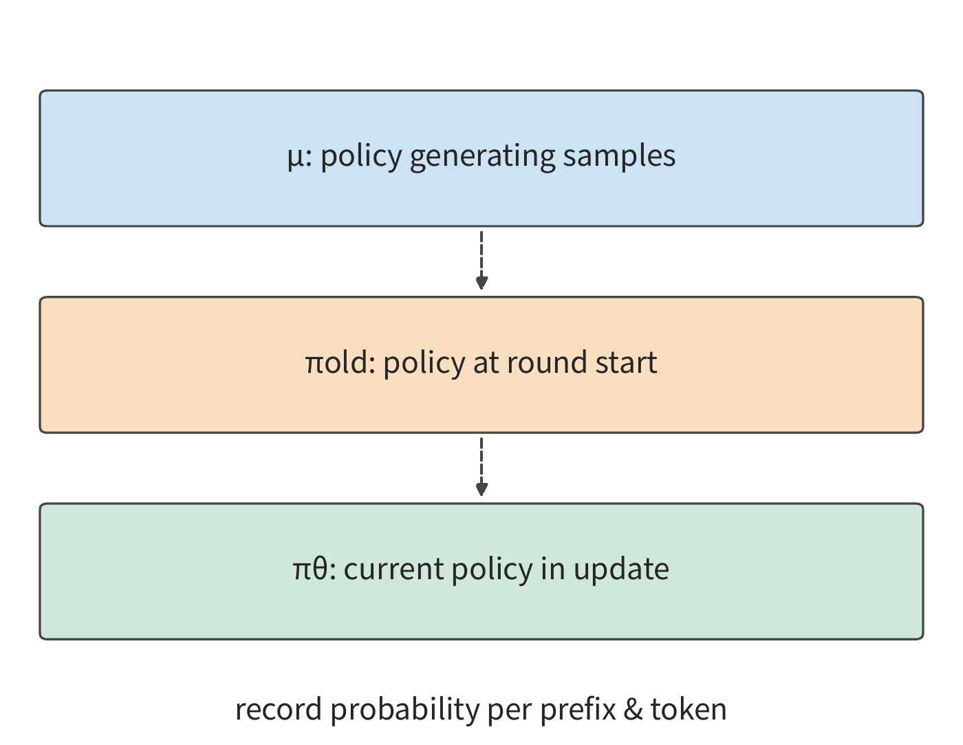
Let \(\mu\) be the actual behavior distribution, \(\pi_{\mathrm{old}}\) the starting policy for this round of optimization, and \(\pi_\theta\) the policy currently being optimized. The starting policy is updated each optimization round, while the reference model used for KL-divergence regularization remains fixed. For the same token and prefix, at positions where all three probabilities are defined and the denominators are nonzero, the probability ratio satisfies

\[ \frac{\pi_\theta}{\mu} =\frac{\pi_\theta}{\pi_{\mathrm{old}}} \frac{\pi_{\mathrm{old}}}{\mu}. \]

The first term on the right describes the probability change brought about by this round's parameter optimization, and the second term describes the discrepancy between the actual sampling distribution and this round's starting policy, which may include both policy version lag and differences from sampling configuration or cross-engine computation. If both the behavior policy and the current policy give this token a log probability (logprob) of \(-3\), the total ratio is 1; if a mistakenly recomputed log probability is used in place of the value originally recorded by the behavior policy, and it comes out as \(-3.25\), the ratio becomes \(\exp(0.25)\approx1.28\). The parameters have not changed, yet the sample weight has increased by about 28%. Retaining the behavior probability lets the training side distinguish policy change from computational discrepancy.²³

Even if weights are synchronized before every round, the second term still need not equal 1. The generation side typically decodes token by token and reads from the KV cache, while the training side feeds the whole trajectory in parallel, recomputing the probability at each token position before backpropagating. Different attention implementations, reduction order, batch shape, or weight/KV precision can all make the logprob differ for the same weights and same prefix. Section 5.2.4 already measured one such case: reducing the same row of input over different numbers of segments produced sums of squares differing by 166 ULPs, and the number of segments in turn depends on the batch size at the time. The forward computation is where the two sides first diverge; the backward pass then carries the loss discrepancy constructed by the training forward pass into the gradient. MoE's discrete routing further amplifies this discrepancy, as the next subsection will show.

Part of the second term also comes from sampling configuration: the behavior probability is computed according to the actual sampling rule. Temperature scaling, top-k, or top-p truncation change the model's raw softmax distribution, so the transformed probability and the sampling configuration should both be saved. The training side must reconstruct the input using the corresponding tokenization, chat template, position numbering, attention mask, and EOS/truncation position in order to compute the probability ratio for the same event.

In updates such as proximal policy optimization (PPO), the probability ratio determines the weight the advantage carries in the gradient, and also participates in the clipping decision: when the probability ratio deviates from 1 beyond a set range, clipping truncates its contribution to the gradient. If an implementation discrepancy is mistaken for a parameter update, a sample's contribution may be wrongly amplified or suppressed, and clipping may be triggered incorrectly; if a sequence-level probability ratio is used, the per-token logprob differences also sum together. Longer trajectories therefore accumulate more probability discrepancy, making updates more prone to fluctuation.²³

Importance weighting uses the probability ratio to adjust the contribution of already-sampled events, so the sampling distribution must cover the target events. Tokens excluded by truncated sampling cannot be recovered through the probability ratios of existing samples; when the distributions differ too much, the variance of the weights also grows. Clipping can bound extreme weights but introduces bias, and clipping the two factors separately produces a different loss than clipping the combined ratio. Asynchronous execution increases the time lag in policy version; the benefit calculation below accounts for both the fraction of usable samples and the execution cycle together.

Example: how high a stale-sample discard rate can an asynchronous pipeline tolerate? Each batch takes 40 s to generate, 16 s to learn, and a weight synchronization that blocks both sides takes 4 s, giving a synchronous cycle of 60 s. If generation and learning use independent resources while the weight synchronization still occupies 4 s exclusively, the asynchronous steady-state cycle is \(\max(40,16)+4=44\) s.

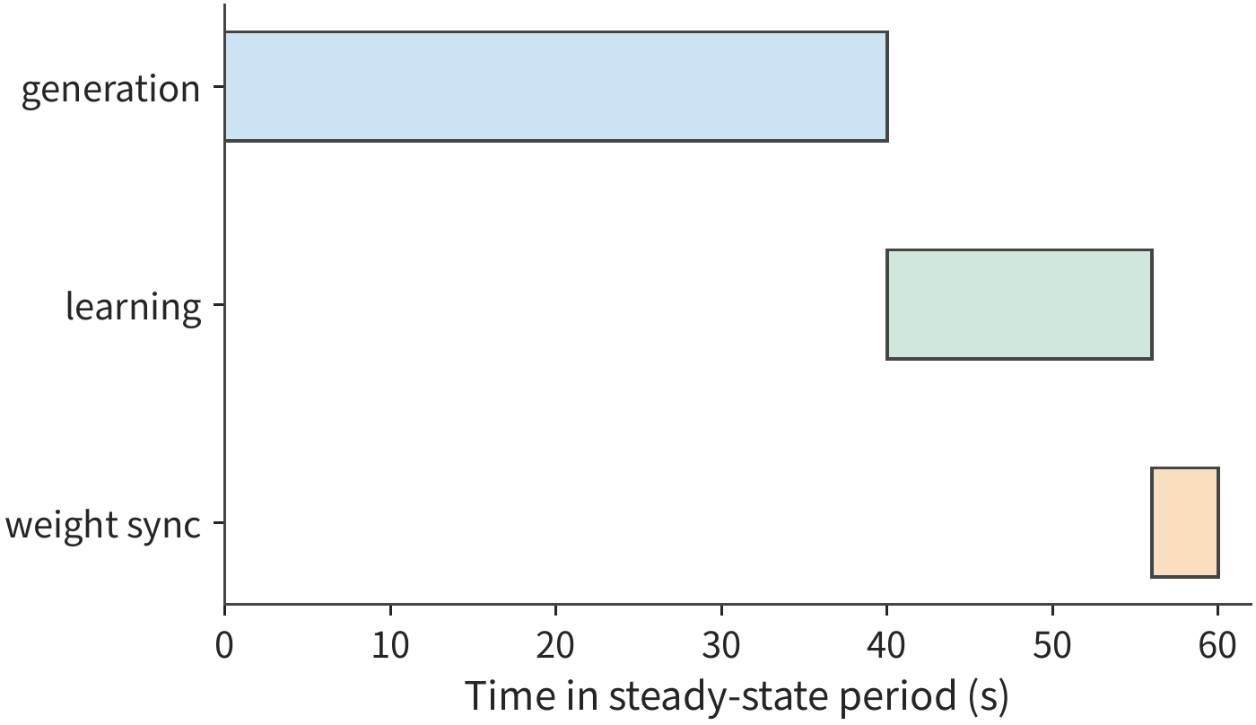
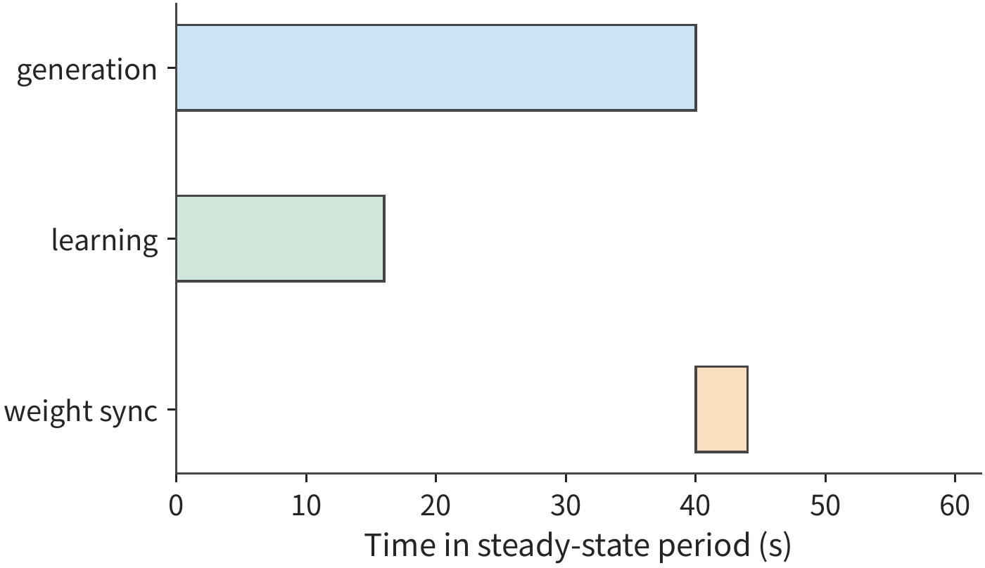
Moving from the synchronous execution in Figure 10-42 to the asynchronous execution in Figure 10-43 reduces the time the learning and generation sides spend alternately waiting for each other. But generating earlier also means samples may use older weights, so the discarded samples must still be subtracted.

If each batch originally has \(B\) equivalent trajectories, and after asynchronous execution a fraction \(q\) of them are retained for training, then the effective sample throughput of synchronous and asynchronous execution are \(B/60\) and \(qB/44\) respectively. For asynchronous execution to be faster requires

\[ q>44/60=11/15\approx73.3\%. \]

At \(q=0.8\), effective sample throughput improves by about 9%; at \(q=0.7\), even though each batch finishes earlier, effective sample throughput actually decreases by about 5%. Therefore, when computing the benefit of asynchronous execution, the samples discarded for having too stale a policy version must also be subtracted.

The generation stage in the figure is drawn as one continuous block of work. The longer the trajectory, the more likely this block is to span a parameter update or encounter an interruption, so beyond filtering completed samples, one must also consider how to continue an incomplete trajectory. Long trajectories also lengthen the time gap between generating a sample and training on it. KV is the result of executing a prefix under given weights: when resuming with the same weights, the saved KV can continue to be used, but after a weight change the prefix must be re-executed to regenerate the corresponding KV. Qwen3-8B's 8K BF16 KV occupies 1.125 GiB; saving and retrieving the KV cache requires storage space and transfer time, while rebuilding the KV cache requires re-executing the prefill computation. The recovery scheme is chosen by comparing retrieval time against rebuild time accordingly.

If interrupted trajectories are always discarded and resampled, longer trajectories are more likely to be discarded simply because they take longer to execute. Let \(\lambda\) be the interruption rate during generation; the probability that a trajectory of duration \(t\) completes generation without interruption is \(e^{-\lambda t}\), and as \(t\) grows, the proportion of data reaching learning falls. Recording generation progress and policy version per token allows generation of the same trajectory to resume after recovery, reducing this length bias introduced by system interruption. Section 11.3.3 shows how a trajectory's model-side and environment-side state survive an interruption.

Making training and deployment use the same path is already seen in real models. DeepSeek V4.1 folds the sparse access and recovery method used at deployment time into training. Sparse attention uses 64K sequences from the very start of training, and post-training adds layer-level candidate limits, so training and inference use the same search domain; quantization-aware training (training that simulates the error of low-precision quantization) lets the model adapt to FP4 main KV; only a limited length of input is replayed to rebuild the decoder's SWA state, and this process is also simulated in post-training. The model thereby learns to use the representation and local state actually provided by the deployment path.²⁸

10.5.4 Expert Routing Replay and Training-Serving Consistency

MoE turns the numerical differences of Section 10.5.3 into further discrete path differences: even with identical weights, numerical computation differences between the generation side and the training side can change expert selection. Because expert selection is discrete, a small numerical change can push a token onto a different computation path. Take the top-2 experts by score as an example: when the top three expert scores are 0.500, 0.301, and 0.300, the choice is expert 1 and 2; if the third score changes to 0.302 because of a different computation order, the choice becomes expert 1 and 3. A very small score change can make the computation switch to a different expert's weight matrix, and the impact can keep propagating through subsequent layers.

Routing replay records the logical expert IDs selected during generation. During training, experts are selected according to these IDs, and the routing scores, expert outputs, and gradients are then computed with the current weights. The sample, token position, and layer number together locate this record. This way, generation and training go through the same discrete expert path, while the numerical computation continues to reflect the current parameters.

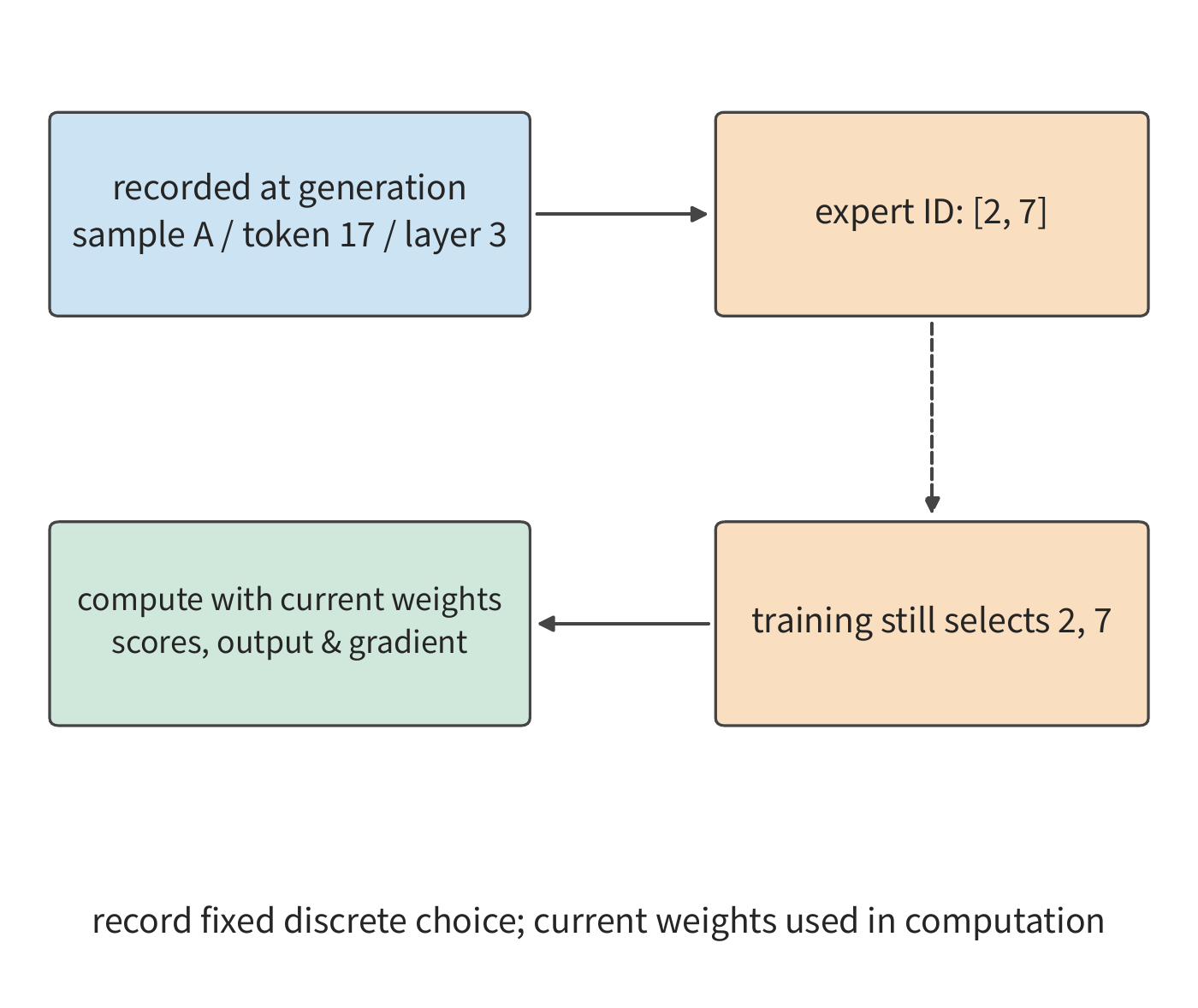
First, calculate how much space this record occupies. Qwen3-30B-A3B's 48 layers each record the IDs of the top-8 experts by score. For 8,192 tokens, storing each expert ID in the uint16 format (an unsigned integer occupying 2 bytes) gives a size of

\[ 8192\times48\times8\times2=6\ \mathrm{MiB}. \]

Using the int32 format, which occupies 4 bytes per integer, gives 12 MiB. The record must also move together with the token: sequence packing changes a token's position, context splitting changes which card a token resides on, and recomputation reads the same layer's record again. Only by letting the ID and the token's original position go through these transformations together can the training side select the original set of experts.²⁴

Case: the impact of routing replay on probability error, training time, and reward. NVIDIA's published validation report on routing replay (R3, i.e., Rollout Routing Replay) has four groups of on/off comparisons, each trained for 100 steps. With replay turned on, the median log-probability error recorded in the logs decreases each time, the median total per-step time is slightly longer, and training reward shows no consistent improvement. Replay reduces routing divergence, but saving the record and executing the replay also adds time. When comparing the two schemes, observe the probability error, training time, and performance on a fixed evaluation task separately.²⁴

Under the same weights and the same batch of tokens, the logprob difference between the generation side and the training side reflects the impact of computation path and sampling definition; MoE's expert IDs indicate whether the discrete routing is consistent. Whether the numerics are consistent, and how far the sampling policy lags behind the current policy, together determine the effective number of training samples.

RL organizes generation, environment verification, and parameter updates into a single, complete feedback process. The generation side provides sampling probabilities and expert selections; the training side organizes updates based on these; resource scheduling then arranges the overlap of the various stages. Connecting this information end to end makes it possible to optimize data handoff, execution consistency, and resource utilization simultaneously. This section's asynchronous cycle and routing replay examples quantify, respectively, the waiting time saved and the record-keeping cost added; the overall feedback loop is ultimately evaluated by effective samples and training progress.

10.6 From System Scheme to Deadline and Hardware Selection

10.6.1 Aggregate Capacity, Per-Step Latency, Stalls, and Recovery

The following brings together the calculation of the completion time for the training task introduced at the start of the chapter. Both schemes process 100B tokens, with each step consisting of 384 sequences of 8,192 tokens, for a total of 31,790 training iterations. Let the per-step training time \(t_s\) already include per-card computation, communication waiting, and input waiting; let \(L\) be the additional time proportion for saving and recovery; and let \(T_0\) be the planned stall. The chapter's first-order completion time model is then

\[ T_{\mathrm{finish}}=T_0+\left\lceil\frac{D}{b}\right\rceil t_s(1+L). \]

Each term comes from a different level of analysis in this chapter: analyzing a tensor's lifecycle confirms whether GPU memory is sufficient; analyzing the critical path yields \(t_s\); the checkpoint model gives \(L\); and the planned stall is \(T_0=5\) days. Bringing these results together makes it possible to compare the completion times of the two schemes; the totals in the table are computed from unrounded values.²⁷

Design item	32-card scheme	48-card scheme
Number of eight-card hosts	4	6
Full-group ZeRO-3, per-card single-sequence accumulation count	12	8
Estimated per-card GPU memory usage / GiB	13.8	12.5
Available per-card GPU memory / GiB	22	22
Per-card computation per step / s	78.3	52.2
Per-step ZeRO-3 link time (PCIe 4.0 x16) / s	17.9	12.0
Per-step communication waiting / s	0.08	0.08
Per-step time waiting for input data / s	0.5	0.5
Per-step training time (including 0.5 s input waiting) / s	78.9	52.8
Additional time for saving, redo, and recovery	1.02%	1.08%
Base training time / days	29.0	19.4
Including save/recovery and 5-day reserve / days	34.3	24.6

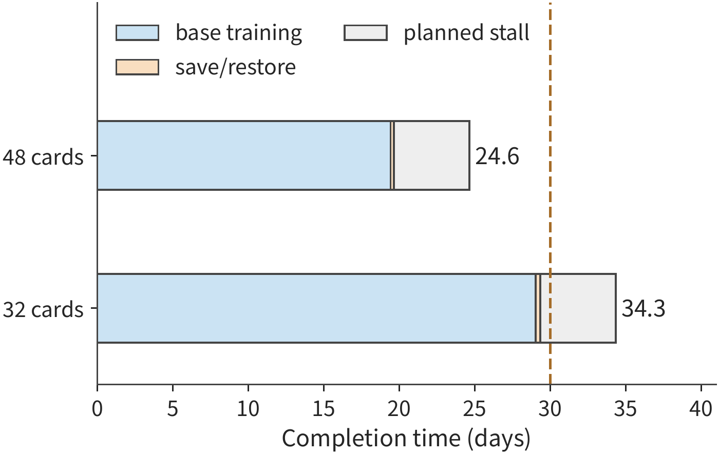
In Figure 10-45, the two schemes have the same planned stall, and saving and recovery occupy only a very small segment. The main difference lies in the blue base training time: the 48-card scheme distributes the micro-batches across more cards for parallel processing, substantially shortening this segment.

Under this set of design conditions, the 48-card scheme is chosen. Both satisfy the capacity requirement; the 32-card scheme's completion time exceeds 30 days and is excluded; the 48-card scheme completes in about 24.6 days, leaving about 5.4 days to spare. The main value of adding more cards is reducing the training work each card carries; the additional failure cost offsets only a small fraction of this benefit.

10.6.2 The Feasibility Range for a 4090 Cluster

Figure 10-45 gives a remaining margin of about 5.4 days. Amortizing this margin back over each iteration shows how much additional waiting each step can tolerate, which yields a performance target usable for actual tuning. The 48-card scheme's per-step training time must satisfy

\[ t_s\le\frac{25\times86400}{31\,790\times(1+0.0108)}\approx67.2\ \mathrm{s}. \]

This scheme currently achieves about 52.8 s, leaving a margin of about 14.4 s per step. Fixing the per-card computation time at about 52.2 s and input waiting at 0.5 s, the total communication waiting can be at most about 14.5 s; per the overlap analysis in Section 10.3.3, only about 0.08 s is currently exposed. Even if prefetching failed completely, exposing the full 12.0 s link time, each step would take about 64.8 s, still within the upper bound.

The 32-card scheme, on the other hand, needs higher per-card computation efficiency. After subtracting recovery, 0.08 s of communication, and 0.5 s of input, about 66.7 s can be allotted to per-card computation, while 40% efficiency requires about 78.3 s. The same amount of work requires raising per-card computation efficiency to about \(40\%\times78.3/66.7\approx47\%\), already higher than the 43% maximum reported for Llama 3. So the two improvement paths can be compared directly: adding two more hosts, or raising per-card computation efficiency on the existing cards from 40% to about 47%.

The communication budget must also be grounded in the physical interface. The 12.0 s link time in Section 10.3.3 assumes one 200 Gbit/s NIC per card. If the eight cards in a single host share just one 200 Gbit/s NIC, the edge of the ring collective communication entering and leaving that host must carry the full send/receive volume for every card on it (the cut set from Example 7.1 in Chapter 7); in the 48-card scheme, about 385 GB per step must pass through this single 25 GB/s NIC, giving a link time of about 15.4 s, which exceeds the 14.5 s communication ceiling. The link time per micro-batch is about 1.92 s, still shorter than the 6.53 s of computation, so when prefetching is effective, only the first and last communications are exposed; but once prefetching fails, each step takes about 68.1 s, and the scheme misses its deadline. With one NIC per card, the 12.0 s stays within the ceiling even if fully exposed. The difference between the two configurations is that a shared NIC bets on-time completion on overlap, while one NIC per card does not depend on overlap.

In this way, the performance target maps onto a concrete execution process: each step allows at most 67.2 s, of which computation needs about 52.2 s, leaving the rest for communication and input waiting. When tuning, first shorten whichever segment of the critical path exceeds budget; if GPU memory is already sufficient to hold the required tensors, there is no need to do extra work just to save memory.

10.6.3 Bottlenecks and Choices After Hardware Replacement

When replacing accelerators, the budget from the previous subsection can still be used to judge which segment faster computation will shorten, and which segment lower bandwidth will lengthen. A new accelerator changes per-card computation, capacity, and interconnect all at once. Splitting the original per-step time into computation, communication waiting, and other parts makes it possible to judge how much value a given piece of hardware change has. Let \(f\) be the proportion of the original per-step time occupied by a given resource, and let its processing capability change to \(r\) times the original, with all other execution and dependencies held fixed. Then

\[ \frac{T'}{T}=1-f+\frac{f}{r}. \]

This is Amdahl's law applied according to the proportion of each time component. If communication waiting was only 5 ms out of an original 100 ms, halving the bandwidth changes the total to \(95+10=105\) ms; if communication originally accounted for 50 ms, the same halving gives \(50+100=150\) ms. The first task's time increases by 5%, the second by 50%, because the original proportion of time spent waiting on that resource differs by a factor of ten.

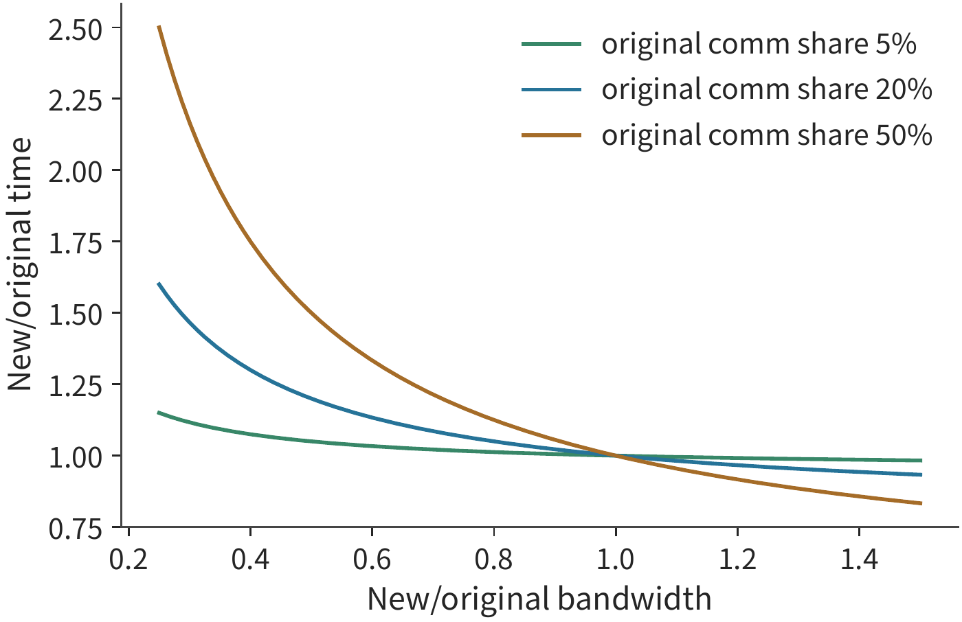
In this chapter's 48-card scheme, the exposed communication is only about 0.08 s, about 0.14% of each step. If PCIe bandwidth is halved, the link time per micro-batch rises to about 3.0 s, still shorter than the 6.53 s of computation; the exposed portion doubles to about 0.15 s, and the per-step time rises from about 52.8 s to 52.9 s — almost unchanged. If per-card computation efficiency drops from 40% to 30%, per-card computation time becomes about 69.6 s, and with communication and input included totals about 70.2 s, exceeding the 67.2 s target. For this scheme, it is per-card computation efficiency, not bandwidth, that determines whether the deadline can be met; bandwidth becomes the term with the larger \(f\) in the formula only when prefetching fails and communication is fully exposed.

When comparing A100, A800, H20, or other accelerators, one can substitute their per-card computation time, interface transfer time, and capacity into the same analysis. Among the schemes that satisfy the deadline, further compare accelerator rental, energy, and preparation costs. Whether a stronger figure on a single specification is worth paying for depends on how much completion time or how many cards it saves.

10.6.4 Sensitivity to Model Scale, Data Volume, and Deadline

The preceding sections held the model fixed while comparing card counts and accelerator models. Finally, extend the same method to model scale, and examine how compute grows as the model is scaled up. Using the rough compute formula for dense models, \(F=6ND\), and fixing the data volume at \(D=20\)T tokens, MFU at 40%, and the available execution deadline at \(T\), the number of cards needed to meet the deadline is

\[ p\ge\left\lceil\frac{6ND}{P\eta T}\right\rceil. \]

Figure 10-47 plots the 90-day deadline as a card-count boundary. Once a model scale is chosen, the compute resources above the boundary can complete the work at that efficiency, while those below the boundary need higher efficiency or a longer deadline.

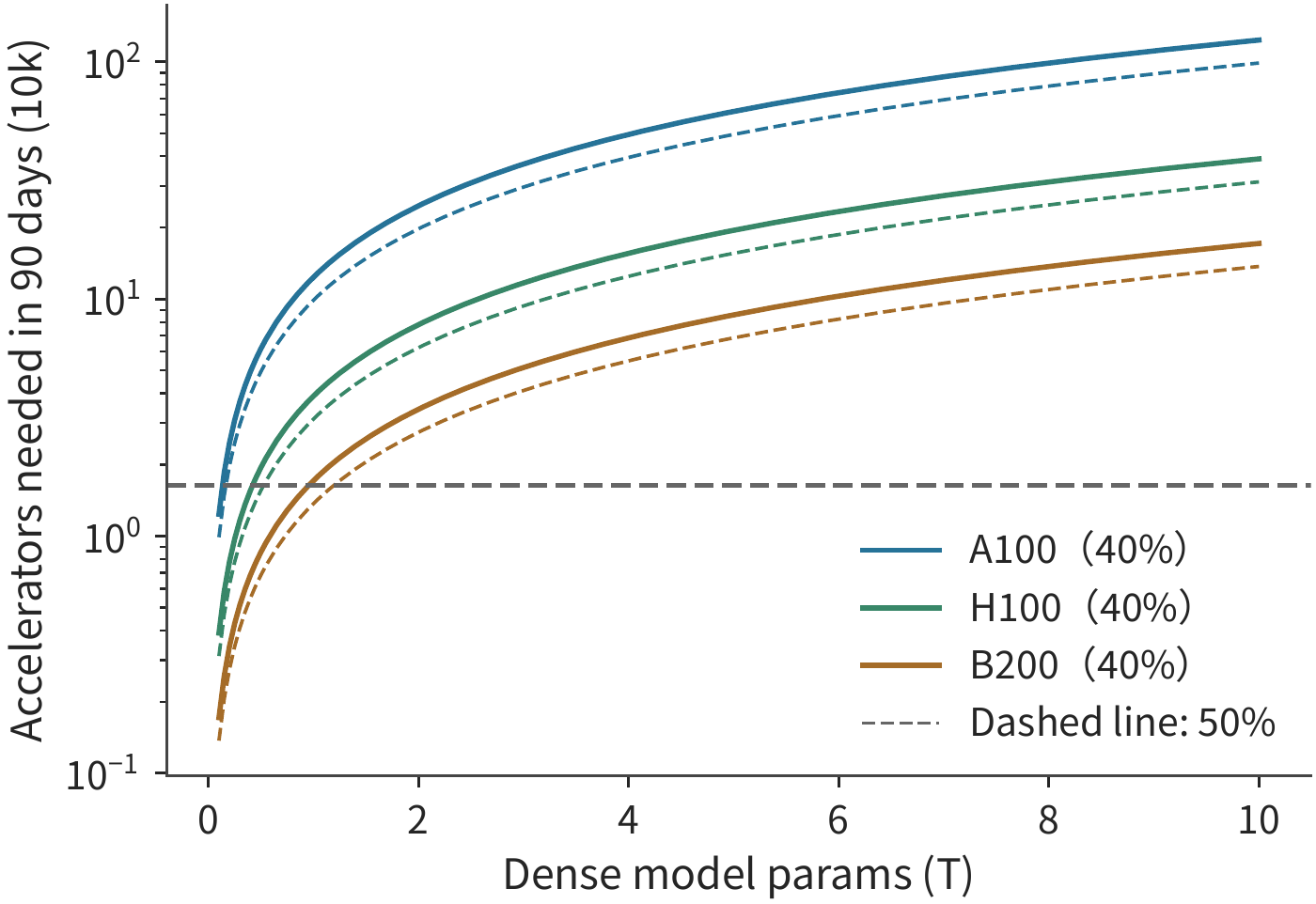
For a 1T-parameter model, 16,384 A100, H100, and B200 cards at 40% MFU need about 679, 214, and 94 days respectively. Under a 90-day execution budget, all three fall below the compute boundary: even B200 exceeds it by about 4 days, requiring an increase to about 17,147 cards. Only when MFU reaches 50% does B200 drop to about 75 days, falling within the deadline, with about 15 days left over for planned stalls and recovery. A 10-percentage-point difference in MFU is what determines whether 16,384 B200 cards can finish training a 1T model within 90 days.²⁵

At a fixed data volume, increasing the parameter count fivefold also increases the compute fivefold; but if the data volume simultaneously satisfies \(D=20N\), then \(F=120N^2\), and increasing the parameter count fivefold increases compute by a factor of 25. The answer to a scaling question is jointly determined by the model and the data. MoE, by contrast, computes the state of all trainable parameters separately from the execution work of the activated path, then places expert exchange on the critical path.

Once the design is complete, one must still check whether long-run execution meets expectations. Public training logs offer a window for observing long-run execution. If training continues from a checkpoint, the newly added tokens for this run equal the cumulative count at the end minus the cumulative count at the recovery starting point; dividing the newly added work by this run's time gives the corresponding long-run rate. This rate can be used directly to check whether the whole system sustains the effective training progress assumed in the design.²⁶

Looking back over the whole chapter: Figures 10-10 through 10-14 explained how data occupies GPU memory and passes through links; Figures 10-17 through 10-36 showed how these operations create waiting and, in turn, affect long-run training; Figure 10-45 then brought all these time components together into the completion time of the task introduced at the chapter's start. State arrangement, execution order, and recovery method are thereby linked into a single design problem. RL changes the source of work into a feedback loop, but still uses the same method to compare resources and effective training progress. The next chapter further discusses how these jobs and stages share a resource pool.

Common Pitfalls

Pitfall: doubling the number of shards halves the training memory peak. Sharding directly shrinks only the resident training state assigned to each card. In the small-model example, resident training state drops from 18 MiB to 9 MiB, but the other tensors and buffers used during execution still occupy about 21 MiB, so the peak drops only from 39 MiB to 30 MiB. What determines the capacity requirement is the total GPU memory footprint at a single point in time.

Pitfall: shorter communication processing time means shorter training-step time. The total processing time of three small buckets is about 4.59 ms, longer than the single whole bucket's 4.55 ms, yet the three can each use a separate compute idle window to complete their transfers. It is the moment at which communication finishes that determines whether it lengthens the training step.

Pitfall: once an asynchronous save call returns, all prior progress can be recovered. In a 50 s failure, the available recovery point depends on which snapshot has already been committed. The same 1 s foreground pause can correspond to 30 s or 10 s of redo work, the difference coming from when the background write completes.

Pitfall: raising generation throughput speeds up RL learning. With generation at 12 sequences/s, verification at 6 sequences/s, and a sample retention ratio of 75%, the learning side receives only 4.5 trajectories per second. Adding generation resources cannot remove the bottleneck at the verification stage; only improving verification capacity shifts the constraint to the training side.

Pitfall: doubling the card count and scaling the batch size proportionally halves the completion time. Once the batch size exceeds the critical batch size, the number of steps needed to reach the same loss no longer decreases appreciably. With a noise scale of two million tokens, scaling the per-step batch size from 3.15 million to about one hundred million tokens (1536 cards) reduces completion time only from 19.4 days to 12.1 days, an acceleration ceiling of 1.64x. Scaling up the batch size is limited by the gradient noise scale; strong scaling, which keeps the batch size fixed and only adds cards, is not limited by it.

Exercises and Experiments

The following ten exercises progress from basic calculations through mechanism analysis to comprehensive design. All conditions needed for the calculation problems are given in the main text; the experiment portions use the accompanying records or data measured independently.

Exercise 10-1 · Basic: training state sharding and per-card peak memory

Change this chapter's gradients to FP32 and compute Qwen3-8B's resident training state. Then find the per-card capacity for eight-card ZeRO-1, ZeRO-2, and ZeRO-3. Assume execution involves 6 GiB of activations and two module buffers of 3 GiB each; compute the peak GPU memory usage both when the two buffers occupy memory simultaneously and when they are reused sequentially.

Exercise 10-2 · Basic: what per-card computation efficiency is needed to complete training on schedule

Using this chapter's training task, set the global batch size to 384 sequences and compute the per-step budgets corresponding to 30 days and 25 days. Given 32 cards, first follow Section 10.3.3 to find the per-step ZeRO-3 link time and exposed communication waiting, then add 0.5 s of input waiting; first ignoring recovery, find the minimum per-card computation efficiency needed to complete training within 25 days; then add this chapter's recovery cost. Finally, taking the gradient noise scale as two million tokens, use the relationship in Section 10.1.1 to find the weak-scaling acceleration ceiling, along with the completion times for 96 and 1536 cards under weak scaling and strong scaling; recompute the ceiling after changing the noise scale to twenty million tokens.

Exercise 10-3 · Comprehensive design: choosing a training scheme among capacity, deadline, and accelerator cost

Compare the training completion times of the 32-card and 48-card schemes, along with cumulative GPU-hours used. Raise the peak requirement for per-step activations and temporary buffers from 10 GiB to 20 GiB and re-judge capacity. If the BF16 weight copy is instead saved using the FP8 block-scaled format from Section 10.1.2, recompute each scheme's per-card resident state and capacity margin. If only four eight-card hosts can be rented, separately compute how much the task volume must be reduced, how much the deadline must be extended, or how much the computation efficiency must be raised, in order to complete training. For the experiment portion, choose one route to measure in practice, and replace this chapter's given parameters with the measured values.

Exercise 10-4 · Analysis: how the number of micro-batches and activation recomputation change pipeline overhead

For a four-stage model with a 10 ms forward pass and a 20 ms backward pass, find the ideal utilization for 1, 4, 8, and 16 micro-batches. Using Figure 10-19, explain which dependency the 93–95 ms wait comes from. Then, for eight micro-batches, compare interleaved 1F1B (\(v=2\)) with zero-bubble scheduling (ZB-H1, \(T_B=T_W\)): compute the bubble time for each using the formulas in the main text, compare against the completion times of 298 ms and 283 ms given by the event model, and explain why the interleaved scheme increases the number of cross-boundary transfers. Suppose each layer's reconstructible product for each micro-batch occupies 10 MiB; in the original scheme, four micro-batches have not yet executed backpropagation, and each micro-batch must retain these products for nine layers. Change this so that only the product needed for one micro-batch in one layer is reconstructed at a time, and released immediately after use. Compute how much less data the new scheme needs to retain, and the size of the working set needed for layer-by-layer serial reconstruction; then discuss how the working set changes when two layers execute backpropagation simultaneously.

Exercise 10-5 · Analysis: how many sequences must be prefetched when the data-preparation process pauses

The 48-card scheme processes 384 sequences per step, with a per-step training time of about 52.8 s; four data-preparation processes each prepare two sequences per second. If one data-preparation process pauses for 60 s, using the training side's average consumption rate, find the minimum number of sequences that must be pre-stored to maintain the original training speed, and how long it will take, once all four preparation processes resume, to refill the prefetch queue back to its pre-pause level. Then, using the 7 GB/s aggregate storage write rate from Section 10.4.3, find the minimum save interval that avoids a write backlog for a checkpoint of about 115 GB.

Exercise 10-6 · Analysis: checkpoint save frequency and failure redo cost

Using this chapter's first-order approximation model, derive the optimal save period, and compute the time overhead caused by checkpoint saving and failure redo for a 1024-card job at save intervals of 300, 900, and 1800 s. Add a shared interruption that occurs once a day and affects the whole job simultaneously, and recompute the failure rate and the optimal period. Then, treat the loss-spike rollback that occurs on average once every seven days as a shock affecting the whole job simultaneously, add it to the 48-card model, and recalculate the optimal save period and the additional time proportion at a 600 s interval. For the experiment portion, inject failures both before and after a submission, and compare the recovery point and the work that must be redone.

Exercise 10-7 · Comprehensive design: RL stage ratios and effective sample throughput

Let the processing rates of the generation, verification, and learning stages be 12, 6, and 8 sequences/s respectively, with a post-verification sample retention ratio of 75%; compare the benefit of doubling the capacity of just one stage at a time. Also adopt a cycle model with 40 s of generation, 16 s of learning, and 4 s of weight synchronization. Assuming the number of samples generated per batch is the same constant throughout, compute the effective sample throughput under asynchronous execution when the sample retention ratio is 80% and 70%, and compare against synchronous execution with no sample dropping; the result can be expressed as the fraction of a batch processed per second. For the experiment portion, trace one batch of samples' identifiers, rewards, effective loss positions, and the recipient's weights.

Exercise 10-8 · Analysis: routing records and their correspondence with samples

Suppose a sequence contains 8K tokens, the model has 48 layers, and each layer selects 8 experts for each token. Compute the record capacity required using uint16 and int32 encoding for the expert IDs, respectively. After packing two sequences together and then splitting them along the context into four parts, describe how the expert IDs get reordered along with the tokens. Construct an example where a token's position is misaligned, explain how the training side would then use the wrong expert, and design a check to locate this error.

Exercise 10-9 · Analysis: how communication, computation efficiency, and input waiting affect the training deadline

In this chapter's 48-card design case, separately halve the PCIe bandwidth (considering both the case where prefetching remains effective and the case where it fails completely), lower per-card computation efficiency to 30%, and raise input waiting to 5 s; recompute the training completion time in each case, and judge whether the deadline can still be met. Then add independent fluctuation with a 5% standard deviation to each card's computation time, find the expected per-step time for the 48-card scheme, and judge whether this scheme still meets the deadline. Assuming all of the above degradations happen simultaneously, but extra resources can restore only one of them to its original value, compare how much critical-path time can be recovered by restoring each item individually. Then choose a hardware specification or execution record, and replace one of this chapter's given inputs with a sourced value.

Exercise 10-10 · Comprehensive design: how many accelerators are needed, and at what cost, to meet a training deadline

For dense models with parameter counts of 1T, 5T, and 10T, use \(6ND\) to compute the training compute under two data-volume regimes: training data fixed at 20T tokens; and training token count satisfying \(D=20N\). Then, at MFU levels of 40% and 50%, find the minimum number of A100, H100, and B200 cards needed to complete training within 90 days and 180 days for each case. Compare, in cumulative GPU-hours, two schemes that both meet the deadline, and explain how preparation time and recovery parameters would change the conclusion. For the experiment portion, select a public log that marks its recovery starting point, subtract the token count already completed at the time of recovery, and compute the average processing rate of newly trained tokens over the observation period.

Chapter Summary

The memory capacity required for training is jointly determined by the storage format of the state, its allocation across cards, and its lifecycle. ZeRO reduces state replication, recomputation reduces the data that must be saved between forward and backward passes, and offloading moves temporarily unused training state to host memory; all three trade extra computation or transfer for GPU memory space. During execution, data readiness and resource availability together determine the start time, and the latency accumulated along the dependency chain up to the end of the parameter update determines the per-step latency.

When estimating long-term completion time, one must also add the data preparation, checkpoint saving, and failure-retry time not included in the per-step latency. A checkpoint saves both the optimizer state and the location of already-completed training data; the save period balances the write cost during normal operation against the retry cost after a failure. Synchronous training is further affected by three practical factors: whether batch size can scale with card count is determined by the critical batch size, per-step latency is determined by the slowest card, and the rollback rate from loss spikes enters the save-period model together with the hardware failure rate. RL further requires tracking sample identity, policy version, and behavior probability, and aligning the numerical paths of generation and training. Online sampling makes the data follow the changing policy, OPD lets teacher supervision cover the prefixes the student actually generates, and cross-engine execution must also guarantee training-serving consistency. Once data distribution shift and execution error are controlled, one can judge how stage overlap speeds up learning based on effective sample throughput and task evaluation.

In this chapter's design case, both 32-card and 48-card RTX 4090 configurations can accommodate the training state, but given the same training objective and execution efficiency, the completion times are about 34.3 days and 24.6 days respectively. The 48-card configuration meets the 30-day deadline, with an upper bound on per-step training time of about 67.2 s; the ZeRO-3 per-step link time of 12.0 s is mostly covered by computation, and even if fully exposed it would not exceed this upper bound. This conclusion follows from a continuous derivation of capacity, execution, and recovery; the same analytical model also gives the critical values at which the scheme can or cannot meet the deadline as efficiency, communication, and failure conditions change.

---

1. Critical batch size recomputation and comparison with a noise scale of twenty million tokens. The definition of gradient noise scale is given in Equation (2.8) of the empirical model for large-batch training; the step-count-vs.-samples relation, Equation (5.1), the definition of critical batch size, Equation (5.2), and the one-to-two-million-token range at convergence are given in the Scaling Laws paper. \(B_{\mathrm{noise}}\) is the value used in this example and has not been measured on this chapter's model; neither weak scaling nor strong scaling includes changes in parallel efficiency. ↩↩

2. The mixed-precision training paper (loss-scaling mechanism, scaling factors from 8 to 32K, FP16 representable range), the FP8 formats paper (E4M3/E5M2 encoding and maximum normal values), the DeepSeek-V3 technical report §3.3 (1×128 activation and 128×128 weight block scaling, promotion to FP32 accumulation every 128 elements, relative loss error below 0.25%). The exponent and mantissa comparison between FP16 and BF16 is given in Section 4.6.1. ↩↩

3. Interleaved event model, zero-bubble event model, DualPipe event model, and the sixteen-micro-batch variants (interleaved, zero-bubble, DualPipe). Bubble formulas: 1F1B and interleaved are given in the Megatron-LM paper (\((p-1)/m\) and \((1/v)(p-1)/m\)); ZB-H1/H2 are given in Table 2 of the zero-bubble paper; the parameter count and activation split for DualPipe are given in Table 2 of the DeepSeek-V3 technical report; the steady-state definition for 1F1B is given in PipeDream. The zero-bubble slot ordering follows the upper half of Figure 3 in the paper for ZB-H1; for the interleaved and DualPipe schemes, the archival text gives only the ideas of chunking and bidirectional feeding, and the slot ordering follows the declared_schedule_rule recorded in each result file; the split ratio of \(T_B=T_W=10\) ms is the value used in this example; the completion times are derived from the event model according to the dependencies, not measured. ↩↩

4. Capacity factor and drop recomputation. The capacity rule is given in Equation (3) of Switch Transformer (per-expert capacity = tokens per batch / number of experts × capacity factor) and in GShard (capacity taken as O(N/E), with overflowed tokens' representation passed to the next layer via the residual connection); bias-based balancing without an auxiliary loss is given in the DeepSeek-V3 technical report. The distribution in which half the experts are 1.5x hot is the value used in this example, giving the same 3:1 ratio as the 96/32 example in the main text. ↩↩

5. Total costs and failure causes are reported in the MiMo-V2.6 Technical Report, Sections 4.1 and 5.5. Per-event timestamps, rates, and rollback notices are in the archived logs; see the case-study memo and recalculation results for the calculations. Costs are estimates obtained by multiplying event intervals by the dashboard's fixed rates, not a separate failure-cost bill published in the report. Rework, detection, and waiting are not separately timed within those intervals, and potentially reusable rollout results are not deducted. ↩

6. Straggler maximum model (σ as 2% of the mean) and (σ as 5% of the mean). The observation that about 0.5% of machines are noticeably slower is given in MegaScale; the mean time between failures of 7.9 hours for a 1024-card job and 47.7 days for an 8-card job are given in the Meta cluster reliability paper, and the per-card failure rate in the save-period section is converted directly from the 1024-card 7.9-hour figure. The standard deviation of per-card computation time and the loss-spike rollback interval are the values used in this example; the expected maximum is obtained by numerical integration based on order statistics, without modeling correlation, periodic jitter, or persistent slow cards. ↩↩↩↩

7. Official parameters and Adam/ZeRO state recomputation; the FP32 gradient variant. This chapter uses the specified five-item state representation; other optimizers and low-precision states must be computed separately. ↩

8. Training deadline and device lower bound and the calendar-time variant. Precision, sparsity, and hardware sources are recorded item by item in the JSON. The 38%–43% BF16 MFU figures are given in §3.3.2 and Table 4 of the Llama 3 report; the PCIe 4.0 interface and absence of NVLink on the RTX 4090 are given on the RTX 4090 specification page. ↩↩

9. CPU FSDP2 four-configuration record. The four configurations on the small CPU model produce parameters consistent with the unsharded reference result; the peak memory allocated during training is 39.16/30.14 MiB. ↩

10. Fill-drain event model, 1F1B event model, retention relationships for GEMM input tensors, selective recomputation. The GEMM inputs use an FP32 reference representation; the reconstructible products for nine layers total 90 MiB, with a maximum per-layer reconstruction working set of 6 MiB. The pipeline diagram uses the intermediate results saved by the save_nonlinear strategy and their send/receive buffers. ↩↩

11. Gradient conversion recomputation, fast-link variant, SuperOffload reading and conversion case, CPUAdam offload record. The conversion path starts from GPU gradient readiness and ends with CPU-readable FP32 gradients; both paths use page-locked host memory as a buffer. GPU conversion throughput uses the RTX 4090's 1008 GB/s memory bandwidth (calculations/configs/hardware.json); CPU conversion throughput uses the eight-channel DDR5-4800 from the Xeon Platinum 8480+ specification, \(8\times4800\ \mathrm{MT/s}\times8\) B \(=307.2\) GB/s; both are upper bounds computed from memory bandwidth. NVLink-C2C at 450 GB/s per direction is documented in the GH200 architecture description. ↩

12. The paper reports per-step latency of 23.66/6.34 s, with scaling efficiency of about 93.3%; this corresponds to the full system scaling experiment with a fixed global batch size. The official MegaScale paper and fixed task, historical configuration, and measurement notes. ↩

13. DeepSeek-V3 technical report, expert exchange and backward bucketing case. The 72 MiB split into three buckets, four-member ring AllReduce, 0.02 ms startup, and three 2 ms gaps are the given input; the configuration of one 200 Gbit/s NIC per card is given in the 4090 cluster configuration analysis, and 400 Gbit/s is given in the ConnectX-7 datasheet. Expert load balancing and routing mechanisms follow DeepSeek-V3; the chunked scheduling follows the linked case. ↩

14. Training workload and length distribution estimation. ↩

15. Training data input and shared storage model, input and save coexistence experiment. The event model uses small-scale parameters to demonstrate how the prefetch queue gets drained when checkpointing and data input share storage; the design case in this chapter uses four data preparation processes, each preparing two sequences/s. ↩

16. Checkpoint layout, ByteCheckpoint, and background save reading, logical resharding computation, 112 GB timeline. ↩

17. DCP recovery record, real text pipeline recovery. The 2,000+6,192 figure is a teaching example illustrating leftover tokens during packing. The DCP small model restores two row-sharded copies into three column-sharded copies plus full state; the parameters, Adam state, random state, and next parameter-update result match uninterrupted training. ↩

18. Asynchronous save and pre-commit failure experiment and no-save/synchronous/asynchronous comparison. The original normal-path API takes about 7.25 ms, with metadata commit at about 48.30 ms; the failure experiment sets a barrier before commit and terminates the process. ↩

19. Save period and Poisson retry model. The precise data volume is 114,670,295,040 bytes; at a write speed of 7 GB/s, the save cost is about 16.381 s; the first-order optimum is about 965.29 s, and the Poisson retry model including in-save failures gives about 954.40 s. The 7 GB/s figure is the aggregate write throughput of a single SU in the Good tier of Table 6 in the DGX SuperPOD reference architecture; a 1024-card job interrupts once every 7.9 hours on average, and mean time between failures is inversely proportional to card count, per the Meta cluster reliability paper. The choice in this chapter only needs to distinguish five, fifteen, and thirty minutes. ↩

20. Fixed verl small-model real closed loop, source-code verification of loss and update. The fixed Qwen2.5-0.5B-Instruct training configuration uses single-card NO_SHARD with no_sync=False; the source code and version lock are recorded in the linked material. 0.32/0.30/0.04 are derived using the real length structure with a teaching scalar loss. ↩↩↩

21. Qwen3-8B shared-device peak, Qwen3-235B-A22B sharded weight synchronization. 40 GiB is the given input for GPU memory footprint after sharding/offloading; the two switchover peaks are precisely about 83.256/59.256 GiB, compared against the H100 SXM nominal 80 GB (74.506 GiB). ↩

22. DeepSeek V4 technical report, §5.1 on domain experts and multi-teacher OPD; stage work division follows Chapter 3. ↩

23. RL state, probability ratio, and version, DeepSeek V4 technical report. ↩↩

24. Routing metadata budget, logs and analysis published by the R3 authors. The four paired settings share seed42; reward is a training-batch metric, while logprob is a log-level statistic from the R3 authors. ↩↩

25. Dense scale and deadline, variant with data volume scaling proportionally with parameters. At 16,384 H100s, DP=128, and an 8K sequence length, 41% BF16 MFU is reported in Table 4 of the Llama 3 report. ↩

26. SmolLM3 original training record verification. The SmolLM3 record includes rank stages at 384, 288, and 192, with the final resume actually running for 14,000 steps; the cumulative token count at the endpoint includes prior work. ↩

27. Inputs, derivation, and recomputation for this chapter's design case. The capacity reservation, input waiting, and planned pauses for 32/48 cards are the given input; per-card compute efficiency uses Llama 3's MFU; the model's matrix work comes from the existing training-deadline computation, and the ZeRO-3 communication volume is derived from the same parameter table. The RTX 4090's PCIe 4.0 with no NVLink is given in the RTX 4090 specification page; no P2P support between cards and eight 200 Gbit/s NICs per eight-card host are given in the 4090 cluster configuration analysis; within a single step, only the first AllGather and the last ReduceScatter cannot be hidden, per MegaScale §3.2. Itemized values and independent recomputation are stored in design-case.json. ↩↩↩↩

28. DeepSeek V4.1 official technical report, Sections 1, 2, 3, and 6; fixed conditions and recomputation across chapter sessions. ↩