Operators and Runtime

The same piece of input, just used for one output, is immediately needed for the output next to it: if it stays near the compute unit, the next use can access it directly; if it has already been evicted, it has to be fetched again. A matrix multiplication program has to arrange this order of use, and leave suitable space for inputs and partial sums. Simply changing how many outputs are processed at once, or which block is computed first, changes the number of repeated moves as well as the number of tasks that can execute concurrently.

The matrix multiplication example in this chapter requires about 103 GFLOPs of computation; the input, weights, and output together occupy 128 MiB, yet one tiled implementation reaches about 3 GiB of read/write traffic. Enlarging the output block lets the input be reused more times, cutting the read/write volume in half, but the local storage required per block also grows from 24 KiB to 80 KiB. With these numbers in hand, we can judge whether the time saved by reducing data movement offsets the loss from having fewer blocks running concurrently.

Chapter 4 introduced the accelerator's compute capacity, storage capacity, and data transfer bandwidth. This chapter discusses how programs make use of these resources. Using a segment of an FFN as the running example, we first explain how the host initiates computation and how the accelerator completes the task, then analyze the loops and tiling of matrix multiplication, and how adjacent operators share intermediate results. We then discuss how compilers and runtimes implement these optimizations, and finally compute how much time these optimizations can save for a complete request.

This chapter mainly uses the FFN of Qwen3-8B as its running example: hidden width \(H=4096\), FFN intermediate width \(F=12288\). We first process \(M=1024\) tokens at once, arranging the 4096-dimensional feature vector of each token into rows of input matrix X, and compute one projection \(C=XW\); X, W, and C use BF16, with each element occupying 2 bytes, and the matrix multiplication accumulates in FP32. M denotes the number of tokens processed in one call, with each token corresponding to one row of the input matrix. These tokens may come from a single prefill segment, or from multiple requests within the same batch; during single-request, per-token decode, M is 1.¹

Object	Shape	Size	Role in computation
Input X	\([1024,4096]\)	8 MiB	Each token's feature vector occupies one row; after projection, we get that token's new feature vector
Weights W	\([4096,12288]\)	96 MiB	Shared by the projection computation for all 1024 tokens
Projection C	\([1024,12288]\)	24 MiB	Undergoes subsequent processing such as activation

This chapter revolves around three questions: which work is repeated, which data can be reused, and which computation or waiting determines the total time. In answering these questions, the unit of program execution on the accelerator is the kernel. Analyzing read/write volume, buffer capacity, and kernel count tells us how much work the program does; combining this with the execution order of that work lets us compute how long the program takes.

5.1 Submission, Movement, and Synchronization During Accelerator Execution

Consider first a matrix multiplication whose input and output both reside in CPU memory. The CPU prepares the input, sends it to the GPU, initiates the computation, and then retrieves the result. This process requires the two processors to collaborate. Understanding when each executes independently and when it waits on the other is the foundation for the fusion, pipelining, and graph replay discussed later.

5.1.1 From Framework Invocation to kernel launch

PyTorch is a software framework for expressing tensor operations and organizing model execution. When it calls a matrix multiplication, the CPU first executes framework code: it reads tensor shapes and data types, selects an implementation, prepares addresses and parameters, and then submits the task to the GPU through the runtime and driver. Initiating one kernel execution on the accelerator is called a kernel launch. The runtime is responsible for submitting tasks, managing memory, and synchronizing execution; the compiler generates the accelerator code either ahead of time or on first invocation.

There are three levels here: the operator describes the mathematical work, such as matrix multiplication or activation; the kernel completes this work on the accelerator; the launch is the action by which the CPU initiates this execution. One matrix multiplication can be completed by multiple kernels, and several elementwise operators can also be completed by a single kernel. Consequently, we can optimize either the computation on the accelerator or the overhead of host preparation and task submission.

When CUDA executes a kernel, it launches many threads. A group of threads forms a thread block, and all thread blocks together form a grid. Matrix multiplication typically divides the output matrix into multiple tiles, handing them to different thread blocks for computation; threads within a block cooperate to read the input and accumulate the result. The accelerator schedules thread blocks onto SMs that have available resources. Blocks that finish earlier release resources, allowing subsequent blocks to begin; hence the thread blocks in a grid can execute in batches.

kernel launch is submitted asynchronously. Once the call returns, the CPU has finished this submission, while the GPU executes according to the task queue and dependencies. The CPU can immediately prepare the next task. Only when the CPU needs to use the accelerator's result, or needs to overwrite data the accelerator is still using, does the CPU need to wait for the corresponding accelerator operation to complete.³⁰

This division of labor forms a simple pipeline: the CPU prepares and submits tasks, and the GPU executes them. Large matrix computations run long enough that the CPU has time to prepare the next call; small operators finish quickly, and the GPU more easily drains its task queue and stalls waiting for the CPU to submit the next item. We can therefore accelerate from two directions: reducing the time the accelerator spends waiting on the host, and shortening the kernel's own execution time.

5.1.2 Data Copies Between Host and Accelerator

The CPU can submit the next task in advance, but the accelerator can only compute once its input has arrived. Analyzing the data transfer process first lets us see clearly what work remains after task submission and before computation begins. Besides the H2D and D2H introduced in Chapter 4, GPUs with dedicated memory also frequently copy within that memory; there are three common copy directions:

Name	Copy direction	Typical object
H2D	Host memory → GPU memory	Input tensor of the current batch
D2H	GPU memory → Host memory	Computation result the CPU needs to use
D2D	GPU memory → GPU memory	Fixed input buffer or reordered result

The execution process of the matrix multiplication above is:

CPU prepares input → H2D → GPU computes → D2H → CPU uses result.

Figure 5-1 plots the location of this data in the two memories and the copy directions.

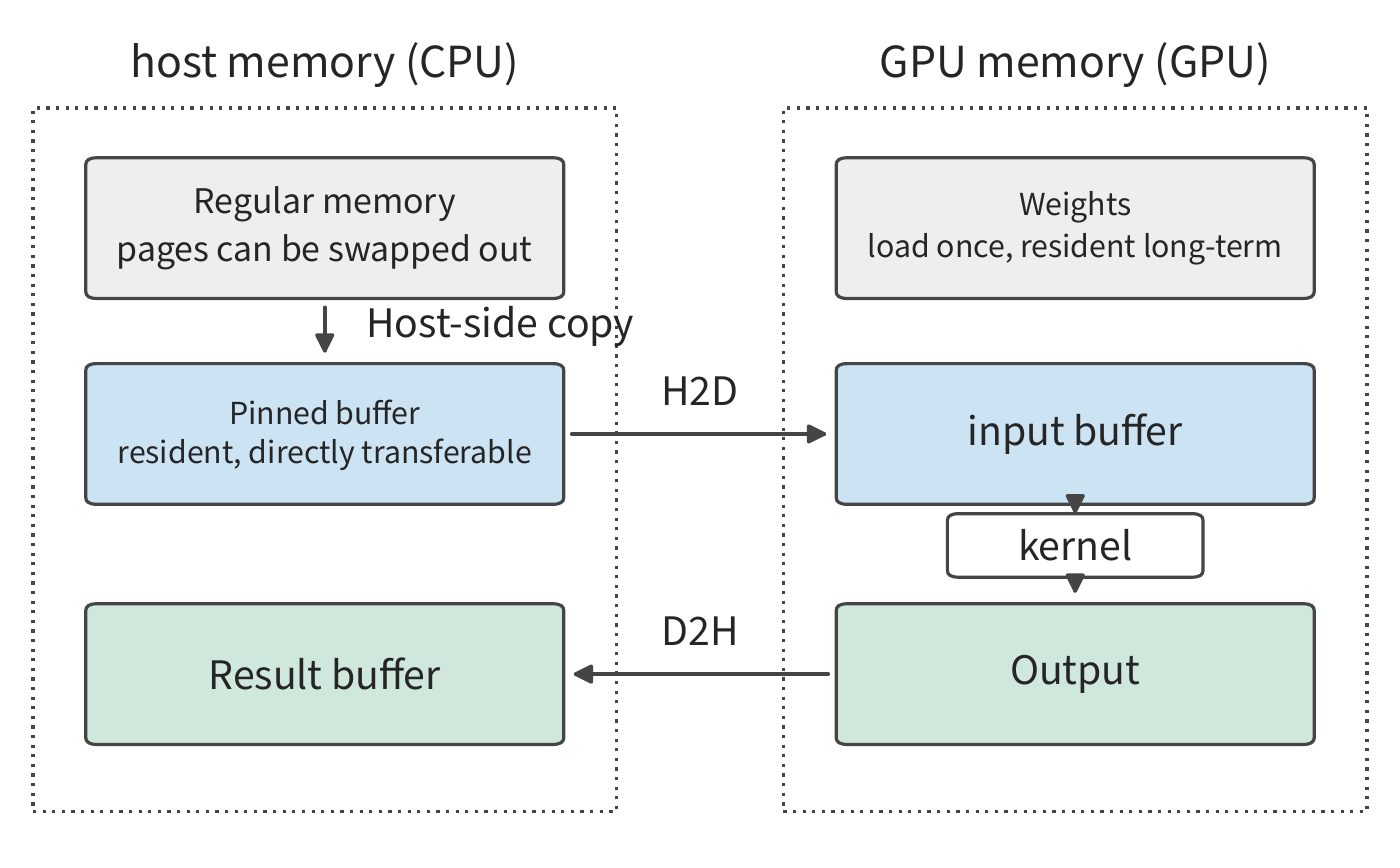
When running a complete model, not every call needs to retransmit all data. Weights, once loaded, can remain resident in GPU memory; inter-layer activations can be read directly by the next kernel; and the KV cache can also continue to be used across subsequent decode steps. If sampling is done on the GPU, the CPU only needs to receive a small number of token IDs. Hence, the number of copies between host and accelerator is not the same as the number of reads within the accelerator: a set of weights may be transferred in only once yet read many times on the accelerator.

Example 5-1: How long does it take to transfer input from the host to the GPU? A BF16 tensor of shape \([8192,4096]\) occupies \(8192\times4096\times2=64\) MiB. An RTX PRO 6000 connects to the host via PCIe Gen5 x16, with a nominal bandwidth of 64 GB/s per direction,³² giving a transfer time of:

\[ T_{\mathrm{H2D}}=\frac{64\ \mathrm{MiB}}{64\ \mathrm{GB/s}}\approx1.05\ \mathrm{ms}. \]

Splitting the input into two 32 MiB tensors, each takes about 0.52 ms, with the total transfer volume unchanged. The benefit of doing this is that the first portion of data can arrive earlier: while the GPU begins computing on the first half of the batch, the copy engine continues transferring the second half. Section 5.3 will further compute the total time once transfer and computation overlap.⁸

The type of host memory also affects the copy process. Ordinary memory pages are managed by the operating system; pinned memory stays resident while in use, making it convenient for the accelerator to move directly. When transferring data from ordinary memory, the runtime often first copies the data into an internal pinned buffer: the CPU copies once, and the accelerator then reads from there. This is the in-host copy on the left side of Figure 5-1. If every batch copies its 64 MiB of data into a newly allocated pinned buffer, an extra host-side copy is performed before H2D. Having the CPU prepare input directly in a reusable pinned buffer avoids this intermediate step and repeated allocation.³⁰

5.1.3 stream, event, and Completion Order

Where data is transferred to determines which processor can use it; when the transfer finishes determines when subsequent computation can begin. After an asynchronous call returns, the copy may still be in progress, so execution order must be used to guarantee that computation does not read input that has not yet finished transferring. A CUDA stream is a sequence of accelerator tasks that execute in order. Placing the H2D copy and the kernel that reads that input in the same stream orders the computation after the copy; the CPU can then submit both pieces of work consecutively.

If the copy and the computation are placed in different streams, an event is used to specify the execution order across streams. The copy stream records an event after the H2D completes, and the compute stream waits on that event before using the input. This waiting occurs within the accelerator task sequence of the compute stream; the CPU can still continue submitting other work.

Figure 5-2 plots two streams and two events on the same timeline.

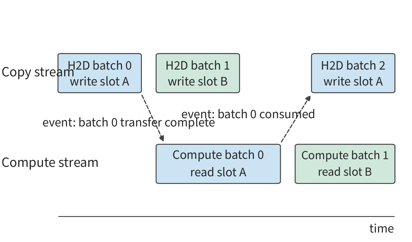
Events can also be used to determine when a buffer can be reused. Suppose the current input is copied from a host buffer into GPU buffer slot A. Once the copy completes, the CPU can write the next batch's input into the host buffer; slot A, however, can only be overwritten once the GPU has finished using the current input. Although the two buffers hold the same batch of data, they become available for reuse at different times.

Buffer	Last user	Subsequent action
H2D host source buffer	Copy engine reads	CPU writes next batch's input
GPU input buffer	Kernel that reads this input	Copy engine writes next batch's input
D2H accelerator source buffer	Copy engine reads	GPU writes new result
D2H host destination buffer	Copy engine writes	CPU reads current result

Therefore, an event should be recorded right after the last read or write, so that the operation that subsequently reuses this buffer can wait on that event. When the CPU needs the D2H result, it can wait on the corresponding event while other unrelated accelerator tasks keep running. The double buffering in Section 5.3 is precisely two such usage sequences interleaved with each other.

This ordering also explains why a program can stall. Every wait points to a specific event; as long as that event is never recorded, the wait never ends — what appears is a stalled program, not merely a slow one. The last-user column for the four buffers in the table above corresponds to four events that are easy to forget to record: if the "consumed" event for the GPU input buffer is missed, the copy engine can never write the next batch. The same applies to cross-stream cycles: stream A waits for an event recorded by stream B, while that task in stream B is itself queued behind work in stream A that has not yet completed, so neither stream advances. Multi-card execution adds one more source: a collective communication call requires every participating card to issue the same call; if even one card fails to issue it, the rest will wait forever for that peer that never arrives (Section 6.4).

When debugging, first check whether the side being waited on is still making progress: if it is still producing results, it is merely slow, and you should return to the timeline in Section 5.1.4 and time it segment by segment; if it is completely stuck, it is waiting on an event that will never arrive — the slow nodes in Section 10.4.5 belong to the former case. Setting a timeout for the wait, and printing the still-incomplete tasks of each stream once it expires, pins down exactly which event is missing.

5.1.4 From Submission Time to Result Availability Time

Connecting the order of copying, computation, and buffer usage is what lets us determine when a result becomes available. Figure 5-3 draws this order as a timeline.

Example 5-2: Why do submission time, accelerator time, and complete call time differ? The input has already been prepared on the host. The CPU submits all tasks within 0–3 μs, and the first accelerator work begins at 3 μs; H2D, the kernel, and D2H take 8, 20, and 4 μs respectively, and the accelerator executes them consecutively according to their dependencies.

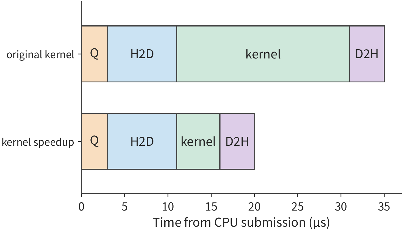
CPU submission takes 3 μs, the kernel executes for 20 μs, and the CPU cannot use the result until 35 μs. If we shorten the kernel's execution time from 20 μs to 5 μs, the result becomes available at \(3+8+5+4=20\) μs. Even though the kernel's speed improves fourfold, the whole execution drops from 35 μs to 20 μs, a speedup of only about 1.8×; the remaining 15 μs is made up of submission and copying.

The three kinds of elapsed time asked about in Example 5-2 correspond exactly to three points at which timing is taken. The measured result depends on where timing starts and stops. Reading the CPU clock before and after an asynchronous call measures the time spent on submission; if you wait for the result before stopping the clock, you measure the time from initiation to completion. A CUDA event marks start and end points within the accelerator's task sequence, measuring the time the accelerator spends on that segment of work. Profiling tools plot host calls, accelerator computation, and copies on the same timeline, making the queueing, dependency waits, and execution following submission visible segment by segment.

The timeline in Figure 5-3 begins once the input is ready. If the program has not yet been compiled, an additional preparation step precedes the timeline: the first call may need to compile code or allocate a workspace. Suppose the first compilation takes 100 ms, and each subsequent execution takes 1 ms; one call then totals 101 ms, and 100 calls total 200 ms, averaging 2 ms per call. The more calls made, the smaller the amortized share of compilation time, while the 1 ms required per execution stays constant. Section 5.5 will use this same method to judge how many repetitions are needed before bucketing (padding inputs to a small number of representative shapes) and specialization (generating dedicated code for a specific shape) become worthwhile.

5.1.5 How a Kernel Executes on an SM

Figure 5-3 drew the kernel as a single 20 μs block; whether it can be shortened to 5 μs depends on what happens on the SM during that time. This section fixes one kernel and walks through five steps — threads, residency, memory access, matrix instructions, and synchronization — to derive how it executes on a single SM. The kernel is the multiply-accumulate block from Section 4.3.2: output block 128×128, with a step of 64 along K; the BF16 A block and W block are each 16 KiB, the FP32 accumulator is 64 KiB, and all three reside in shared memory, forming a working set (the data that must remain in local storage simultaneously during computation) of 96 KiB total. One thread block handles one output block and contains 256 threads. The hardware is an H100 SM: it can hold up to 2048 resident threads simultaneously (i.e., 64 warps, explained below) and 32 thread blocks, with 64K registers (each 32 bits) and 228 KB of shared memory (as written in CUDA documentation, i.e., 233,472 bytes). The kernel uses 128 registers per thread, each load instruction fetches 16 bytes per thread, each warp can have at most 4 outstanding loads, the matrix instruction shape is 16×8×16, and memory latency is taken as 600 ns.²⁹

warp: 32 threads issued together. An SM does not issue instructions thread by thread; instead it groups 32 threads together and issues them as one unit, called a warp. All 32 threads in a warp execute the same instruction, each operating on different data; a single load instruction therefore produces 32 addresses at once. A thread block of 256 threads contains 8 warps. The 32 "lanes" discussed in Section 5.2.3 when analyzing shared memory banks (partitions of shared memory that can service requests independently) are exactly the 32 threads of a warp: how many banks the 32 addresses they issue simultaneously fall into determines how many rounds that instruction occupies the shared memory interface.

Residency and occupancy. For a thread block to be resident on an SM — that is, to remain on the SM available for scheduling at any time — it must simultaneously be allocated thread slots (one per thread), registers, and shared memory. The number of thread blocks each resource category can hold equals the resource total divided by the per-block requirement, rounded down; the resident block count is the minimum across categories:

Resource	SM total	Per-block requirement	Thread blocks accommodated
Thread slots	2048	256	8
Registers	64K	256 × 128 = 32K	2
Shared memory	228 KB (233,472 bytes)	96 KiB working set + 1 KiB reserved per block = 97 KiB	2
Thread block cap	32	1	32

Both registers and shared memory allow only 2 blocks, so 2 thread blocks — that is, 16 warps — reside on the SM. Occupancy refers to the ratio of resident warps to the SM's maximum resident warp count, here 16/64 = 25%. Figure 5-4 draws the three resource categories as three bars: two thread blocks fill the registers exactly, fill shared memory down to only 34 KiB remaining, while the thread slots are only a quarter used.

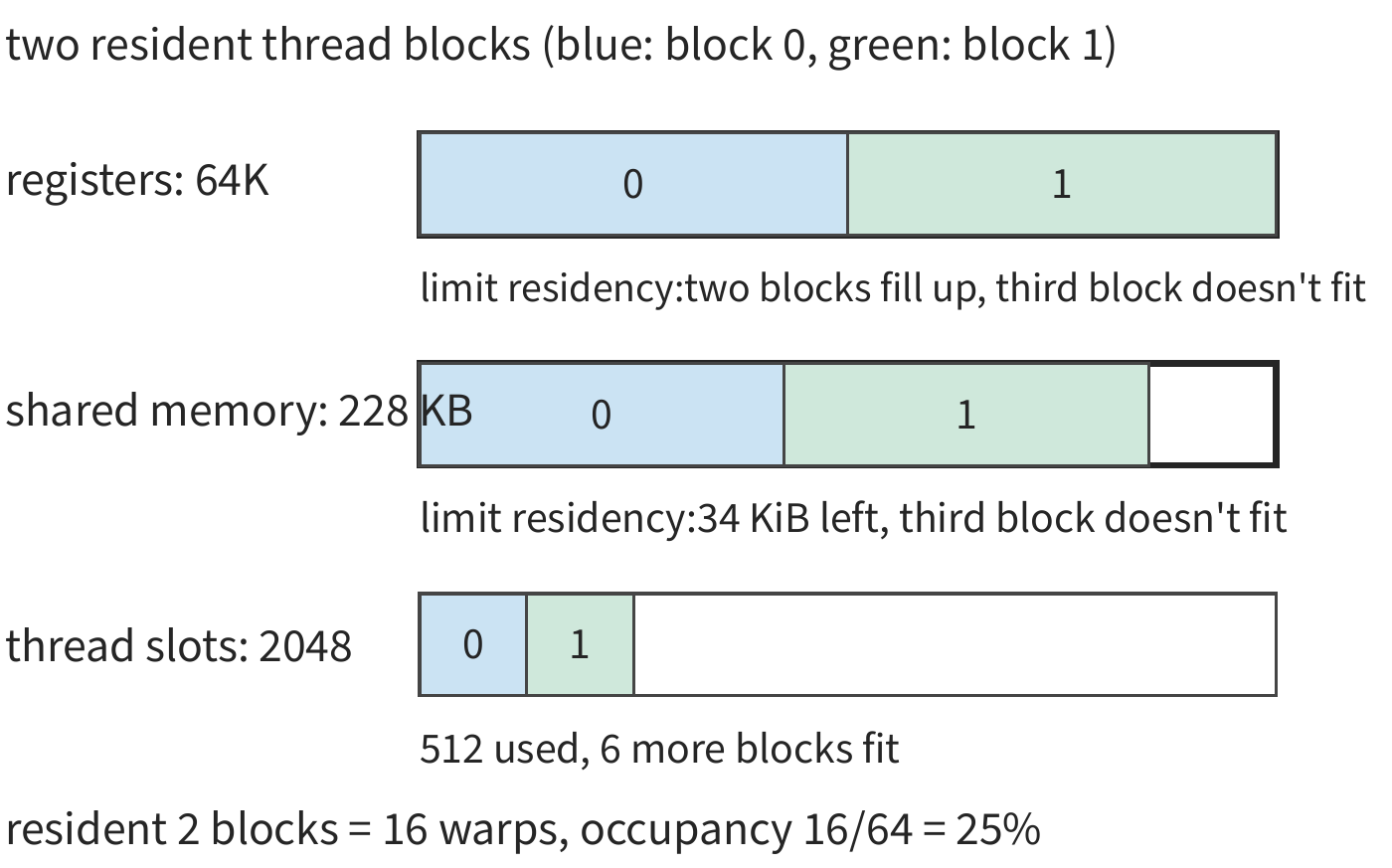
Which resource is worth changing depends on which one is the tightest constraint. Moving the 64 KiB accumulator from shared memory into registers requires each thread to hold an additional 64 FP32 values, i.e., 64 more registers. The shared memory requirement per block then drops to 32 KiB, accommodating 6 blocks; but if each thread originally used only 64 registers, adding the accumulator brings it to 128, and registers still allow only 2 blocks. The resident block count is unchanged; the binding constraint has simply shifted from two resources to registers alone. To let a third block reside, both per-thread registers and per-block shared memory must be reduced simultaneously, or the working set per block must be shrunk.

Latency hiding: resident warps supply in-flight requests. Occupancy matters because independent memory access requests all come from resident warps: with enough requests in flight, when one request is waiting for its return, the interface stays occupied by other requests — this is latency hiding. The Little's Law from Section 4.3.3 gives the in-flight bytes needed to sustain bandwidth: bandwidth × latency. Taking the H100's memory bandwidth of 3.35 TB/s and latency of 600 ns, the whole card needs about 2.01 MB in flight; spread across 132 SMs, each SM must keep about 15.2 KB in flight. We then compute how much the resident warps can supply: one load instruction from one warp has 32 threads each fetch 16 bytes, totaling 512 bytes; each warp can have at most 4 outstanding loads; 16 warps together provide 32 KiB.

\[ B_{\mathrm{need}}=\frac{3.35\ \mathrm{TB/s}\times600\ \mathrm{ns}}{132}\approx15.2\ \mathrm{KB},\qquad B_{\mathrm{have}}=16\times4\times512\ \mathrm{bytes}=32\ \mathrm{KiB}. \]

The available in-flight bytes are 2.15 times the requirement, so even just 8 resident warps (one thread block) would suffice. Section 5.2.2 will encounter the phenomenon where "a bigger block reading less data can nevertheless be slower" — this gives its quantitative form: the larger the working set, the fewer blocks reside, and the fewer in-flight bytes are available; once that falls below the requirement, effective bandwidth drops to available in-flight bytes divided by latency, and no amount of interface bandwidth helps.

Matrix instruction granularity. Section 4.2.1 explained that the matrix unit executes fixed-shape blocks. Here one matrix multiply-accumulate instruction (MMA) has shape 16×8×16: an A tile of 16×16, a W tile of 16×8, and one instruction performs 2×16×8×16 = 4096 floating-point operations. A 128×128×64 block requires (128/16) × (128/8) × (64/16) = 8 × 16 × 4 = 512 instructions, matching the block's 2,097,152 FLOPs. These 512 instructions are split evenly among 8 warps: the output block contains 8 × 16 = 128 output tiles of 16×8, each warp handles 16 of them, issuing 64 instructions total across the four steps along K. MMA instructions accumulate in registers; the block in this section keeps the accumulated result in shared memory, so before and after each K step, these 16 tiles must be moved between registers and shared memory — the accumulator-in-registers scheme from the paragraph above eliminates exactly this movement.

MMA can be issued in two ways. A warp-level instruction is issued by a single warp on its own, with operands first loaded into that warp's registers; Hopper's warpgroup-level instruction is jointly issued by 4 adjacent warps (collectively called a warpgroup), which can fetch operands directly from shared memory and execute asynchronously: the warp that issues the instruction can do other work while waiting for the result. FlashAttention-3 exploits exactly this instruction arrangement to overlap computation.¹⁰

Synchronization: asynchronous copy and barriers. Section 4.4.2 used two input slots to overlap loading with computation, on the premise of knowing the two moments "slot filled" and "slot consumed." On an SM, these two moments are given by a barrier. A barrier is a counter in shared memory: each participant arrives at the barrier after finishing its own step, and once the count reaches a predetermined value, the threads waiting at the barrier are released. Asynchronous copies (copies issued and completed in the background by hardware, without the issuer needing to wait) also arrive at the barrier upon completion, counting by the number of bytes moved in. Each slot is paired with two barriers: the "full" barrier is triggered by copy completion, and computation waits on it; the "empty" barrier is triggered by the end of computation, and the next copy waits on it.

With barriers in place, warps can divide labor: one warp issues only copies (the producer), while the remaining warps only compute (the consumers) — this arrangement is called warp specialization. After the producer warp issues the copy for block j+1, it does not need to wait for it to complete; instead it waits on the "empty" barrier, preparing to write block j+2. Each time a consumer warp reaches the "full" barrier, it proceeds to compute the next block.

Let's first compute the time each of copying and computation takes. Splitting the H100's memory bandwidth of 3.35 TB/s and its BF16 dense matrix peak of 989.4 TFLOP/s evenly across 132 SMs gives each SM about 25.4 GB/s and 7.50 TFLOP/s; the computation below assumes this thread block has exclusive use of its SM's share. One K block's A and W together total 32 KiB, taking about 1.29 μs to copy; the block multiplication is 2,097,152 FLOPs, taking about 0.28 μs to compute. Copying is about 4.6 times slower than computing, because this block performs only 64 floating-point operations per byte moved, while the H100's ratio of matrix peak to memory bandwidth is about 295 FLOP/byte. Figure 5-5 draws four K blocks across two slots using these two time values.

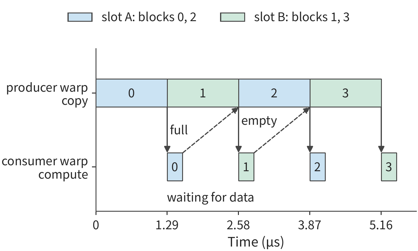
This division of labor is the software implementation of the pipeline from Section 4.2.3. There, the three resources were the matrix unit, the shared memory interface, and the exponent unit; here, the producer warp drives copying, occupying the shared memory interface, while the consumer warp drives matrix and exponent operations, with barriers letting each side wait only at the point of data handoff. FlashAttention-3 is designed exactly this way: a producer warpgroup issues copies of K and V blocks, while two consumer warpgroups alternate between matrix multiplication and softmax, so that one is computing exponents while the other is doing matrix multiplication. Section 5.3.2 will use the same values from here — 1.29 μs copy time and 0.28 μs compute time per block — to derive the total pipeline time, and Section 5.3.3 will expand further on FlashAttention's tiling.¹⁰

Asynchronous bulk copy also imposes a requirement on data layout. Section 5.2.3 will use padding — adding one extra word at the end of each row — to spread out banks; asynchronous bulk copy moves whole blocks according to a tensor descriptor (a structure recording tensor shape and stride) and cannot insert padding between rows, so instead it permutes addresses within a block according to a fixed rule — this technique is called swizzle: the total data volume is unchanged, but requests to the same column still land on different banks.

Mapping to Ascend. The five steps discussed in this section — threads, residency, memory access, matrix instructions, and synchronization — correspond on Ascend to another set of components from Sections 4.2.3 and 4.6.2:

Mechanism in this section	NVIDIA GPU	Ascend
Issuing and division of labor	A warp is the unit of issue for 32 threads; producer and consumer warps divide labor within the same SM	AIC and AIV are each independent cores rather than warps: matrix work executes on the AIC, vector work executes on the AIV, each with its own instruction stream
Residency and capacity	Registers, shared memory, and thread slots determine the number of thread blocks resident per SM	The capacities of L0, L1, and the unified buffer determine how many blocks each core holds at once
Movement and synchronization	Asynchronous copies arrive at barriers, and warps wait on barriers	MTE/NDDMA perform the movement, and BufferID identifies buffers and organizes handoffs

The conclusion above, that "enough bytes are in flight," relies on a 600 ns latency and 4 outstanding loads per warp. Flip condition: if latency rises to 1000 ns and each warp can only sustain 2 outstanding loads, each SM needs 25.4 KB in flight, but 16 warps can only provide 16 KiB, dropping the coverage ratio (available in-flight bytes divided by requirement) to 0.65; closing this gap requires at least 25 warps, i.e., 4 thread blocks, while registers and shared memory only allow 2. At this point, 25% occupancy is no longer sufficient: either the working set must be shrunk to gain more resident blocks, or asynchronous bulk copy must be used so that one thread issues a request for an entire block at once, with in-flight bytes counted by block size rather than depending on warp count.

Exercise 5-1 · Extension: If the output block is shrunk to 64×64, which resource determines occupancy?

Keeping 256 threads and 128 registers per thread, change the output block to 64×64, keep the K step at 64, and keep the accumulator in shared memory. Find the shared memory requirement per block, the number of thread blocks each of the four resource categories allows, and the occupancy, and identify which constraint is tightest. Then recompute with per-thread registers lowered to 64, and state where the constraint shifts to; finally, using a 600 ns latency and 4 loads per warp, check whether the in-flight bytes can still cover the requirement.

5.2 Tiling, layout, and actual memory access for a single operator

A large matrix computation can be tiled the way you'd slice tofu: cut it into pieces sized for convenient processing, then finish them one by one. But the shape you cut has to match what the compute unit can process and how much data can sit nearby. Chapter 4 already showed that hardware matrix instructions support only limited shapes; multiple compute units across the whole accelerator can work on many tiles at once, and within each piece of work, the steps still have to be organized into the small increments the hardware can execute.

Tiling also has to make the data brought in get used more than once. Following Chapter 4's workbench analogy, the current input and the not-yet-finished partial sums need to sit near the compute unit, and only when they're done can that space be freed. If the output tile is too small, the same input may have to be moved repeatedly for different output tiles; if the tile is too large, it takes up more local storage and crowds out other work that could run concurrently. Below, we first trace what data a single output needs, then organize multiple outputs into tiles, and analyze how tile size, access order, and local capacity jointly affect reuse.

5.2.1 Matrix shapes and repeated reads

Let A denote the input X from the start of the chapter, and write the projection as \(C=AW\), where \(M=1024,K=4096,N=12288\). A, W, and C are all BF16, sized 8, 96, and 24 MiB respectively. If A and W are each read once and C written once, only 128 MiB of transfer is needed. To explain why one tiled implementation produces roughly 3 GiB of access, first look at how a single output is computed.

To compute C[i,j], take row i of A and column j of W, multiply corresponding elements, and sum along the K dimension. Then compute C[i,j+1] to the right, switching to an adjacent column of W while A remains the same row. The blue portions of the two computations in the figure are identical.

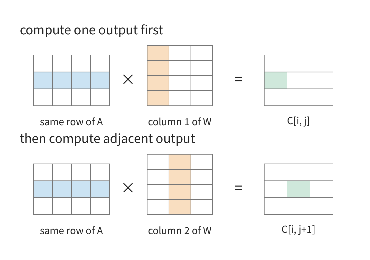
If this row of A stays resident in local storage or cache between the two uses, it can be reused directly; if it has already been evicted, another request has to go to the next storage level. When moving to the next output row, elements of W get reused as well. The same piece of data needs to be used repeatedly across the math operations. How the program arranges these operations determines how many times that data crosses the storage interface.

This section counts at the interface between the working buffer and the next storage level, tallying the bytes the program reads and writes each time. The roughly 3 GiB access figure below is also computed at this interface.²

Writing the elementwise computation in the figure as a loop gives:

for i in range(M):
    for j in range(N):
        acc = 0.0
        for k in range(K):
            acc += A[i, k] * W[k, j]
        C[i, j] = acc

Each pass through the inner k loop produces one output. One multiply-add counts as two FLOPs, so the total computation needed for all outputs is:

\[ F_{\mathrm{gemm}}=2MKN\approx103\ \mathrm{GFLOPs}. \]

The comparison baseline is the read/write volume of three BF16 matrices each crossing the interface once:

\[ V_{\mathrm{once}}=2(MK+KN+MN)=(8+96+24)\ \mathrm{MiB}=128\ \mathrm{MiB}. \]

Here MiB is \(2^{20}\) bytes. Using one read of each input and one write of the output as the baseline, we can compute below how much extra repeated access tiling adds.

Loop order also determines the address pattern of each access. When W is stored row-major, the inner loop above reads W[k,j], W[k+1,j] in sequence, addresses differing by N elements. Switching to i, k, j order, the inner loop instead reads W[k,j], W[k,j+1] in sequence, while reusing A[i,k] across multiple outputs. That way, the data fetched in one contiguous transfer can be used immediately in computation.

However, the new order also has to keep a segment of accumulated output results resident at the same time. If local storage cannot hold these results, each update round may add more reads and writes to the next storage level. Next, we use tiling to bound how much data is held simultaneously, coordinating input reuse with output retention.

5.2.2 Tiled reuse under capacity constraints

First pick a small block of C as the current output to complete, and allocate an accumulator buffer for that \(m\times n\) output tile. Each time, read in a pair of input tiles along the K dimension: an A tile of \(m\times k\) and a W tile of \(k\times n\). The two tiles are multiplied, updating the same output accumulator; when the next pair of input tiles is swapped in, the partial sum already obtained is retained. Only once accumulation along K is complete is the result converted to BF16 and written out. The tile here is organized by software for data reuse, and internally it can still be decomposed into multiple hardware matrix instructions. Tiling itself does not require first copying the original matrix into many separate small matrices — the actual movement is arranged by the executing program.

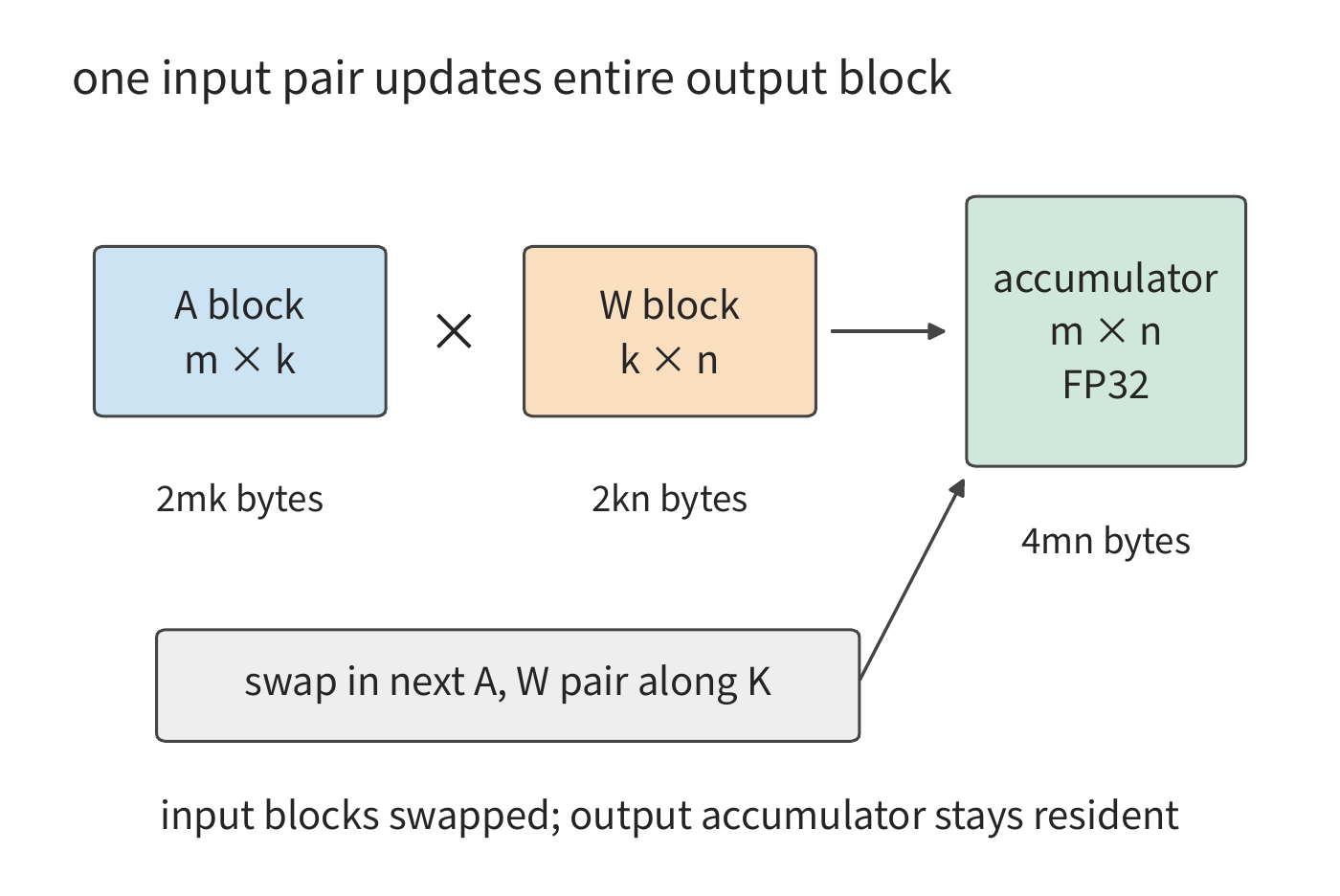
Each element in the A tile can be used for n columns of output, and each element in the W tile can be used for m rows of output. Enlarging the output tile lets one read of data participate in more multiply-adds, but it also requires holding more input and output partial sums.

Example 5-3: How much can enlarging the output tile reduce input reads? In the figure, the A input tile, W weight tile, and output accumulator occupy \(2mk\), \(2kn\), and \(4mn\) bytes respectively. With only one set of input buffers, the local storage requirement is:

\[ S=\underbrace{2mk}_{A\text{ tile}}+\underbrace{2kn}_{W\text{ tile}}+\underbrace{4mn}_{\text{accumulator}}\quad\mathrm{bytes}. \]

Take \(k=32\), first using a 64×64 output tile. The A and W tiles each occupy 4 KiB, the accumulator occupies 16 KiB, totaling 24 KiB. Enlarging the output tile to 128×128, the two inputs each occupy 8 KiB, the accumulator occupies 64 KiB, totaling 80 KiB. Input reuse increases, but the output accumulator grows faster.

Next, compute the read/write volume for the full matrix. Assume each output tile independently reads its own inputs, without considering cache reuse across different output tiles. There are N/n column tiles in the N direction, each of which traverses all of A; there are M/m row tiles in the M direction, each of which traverses all of W. C is written out only once in the end, so:

\[ V=\underbrace{2MK\frac{N}{n}}_{\text{repeated reads of }A}+\underbrace{2KN\frac{M}{m}}_{\text{repeated reads of }W}+\underbrace{2MN}_{C\text{ write}}. \]

A 64×64 output tile divides the output into 16 row tiles and 192 column tiles. The 192 column tiles each read the 8 MiB A once, totaling 1536 MiB; the 16 row tiles each read the 96 MiB W once, also 1536 MiB. Adding the 24 MiB output gives a total of 3096 MiB. This is where the roughly 3 GiB figure at the start of this section comes from.

Switching to 128×128, the number of row tiles drops from 16 to 8, and the number of column tiles drops from 192 to 96, halving the reads of both inputs. The output size is unchanged, and the total falls to \(768+768+24=1560\) MiB. Figure 5-8 compares this benefit against the local storage it occupies.

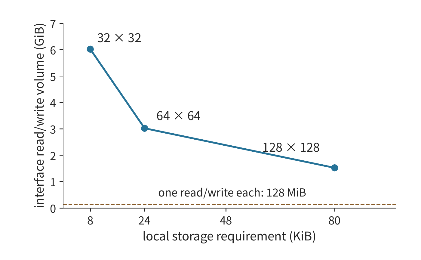
The full figures are below; arithmetic intensity is computed as the FLOPs of the same matrix multiply divided by the interface byte counts above:

Output tile	Local storage required	Access between working buffer and next storage level	Arithmetic intensity
32×32	8 KiB	6168 MiB	15.9 FLOP/byte
64×64	24 KiB	3096 MiB	31.7 FLOP/byte
128×128	80 KiB	1560 MiB	63.0 FLOP/byte

The arithmetic intensity of all three output tiles is far below the 295 FLOP/byte ratio of H100 matrix peak to memory bandwidth given in Section 5.1.5. Looking only at traffic at this interface level, all three tilings sit on the bandwidth-bound side, with matrix unit MFU ceilings of only 5%, 11%, and 21% respectively. Enlarging the output tile pushes arithmetic intensity toward the crossover point, but tiling alone at this level cannot get past it — the remaining reuse has to come from storage levels closer to the compute unit.

Access volume nearly halves, but whether time halves accordingly depends on how much work the accelerator can schedule concurrently. On GPUs, input buffers sit in shared memory, and the accumulator can sit in shared memory or registers. Here we follow the approach of Section 5.1.5: each thread block handles one output tile, with both input buffers and the accumulator in shared memory. Take the RTX PRO 6000's single SM as the hardware: this card is compute capability 12.x, with a per-SM shared memory limit of 100 KB (i.e., 102,400 bytes), with each thread block also reserving 1 KiB.³³

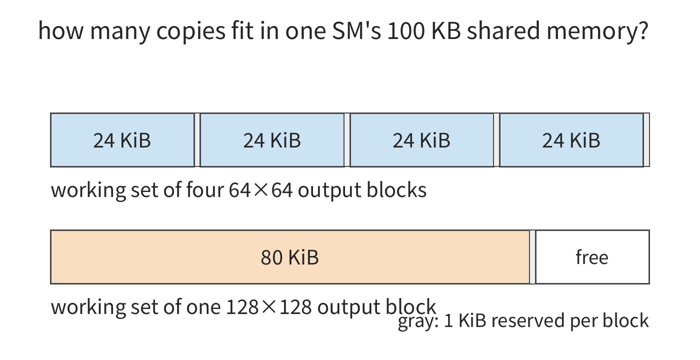
Concurrently resident thread blocks can interleave memory requests: while some blocks wait on data, others keep working. When the concurrently resident working set drops from four copies to one, there is less other computation available to run during memory waits. So while the larger tile reads less data, the effective bandwidth it actually achieves may drop. Section 5.1.5 already worked this out: resident warps supply in-flight memory requests, and when in-flight bytes are insufficient, effective bandwidth falls below interface bandwidth.

Assuming both implementations are bandwidth-bound at this level, with effective bandwidths \(B_{64}\) and \(B_{128}\) respectively:

\[ \frac{T_{128}}{T_{64}}=\frac{1560}{3096}\frac{B_{64}}{B_{128}}. \]

If the bandwidths are equal, time roughly halves; if the larger tile achieves only 40% of the original bandwidth, the time ratio becomes about \(0.504/0.4=1.26\) — a roughly 26% increase in time instead. One can first rule out schemes that don't fit within capacity, then narrow the comparison by access volume, and finally measure actual execution efficiency. Section 5.4 hands this process over to the compiler.

5.2.3 Data layout: spreading concurrent requests across different banks

In the previous subsection, larger tiles read less data but could slow down due to lower parallelism. Parallelism depends not only on how many thread blocks are resident, but also on whether the read requests these threads issue can be served simultaneously. Consider the local storage layout first. Take a 32×32 FP32 scratch tile, whose local storage is divided into 32 banks; each bank supplies one 32-bit word per cycle, and the bank number is the word address modulo 32. Section 5.1.5 already introduced that a warp's 32 threads are 32 lanes; when 32 lanes each read one word from the same row, the requests spread across 32 banks; when reading a column, the row stride is 32 words, so all addresses land on the same bank, requiring 32 cycles.

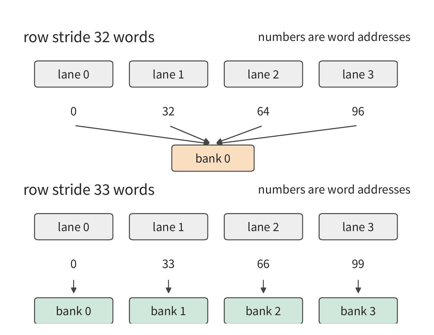
Padding one extra word at the end of each row changes the row stride to 33. The bank numbers for adjacent rows in the same column then increase by one each time, so the 32 requests spread across 32 banks and complete in a single cycle. The space occupied grows from 4096 bytes to 4224 bytes, an increase of only about 3.1%. Neither the effective data nor the number of reads changes, but a column read that originally needed 32 cycles now completes in one.

This extra word at the end of a row is padding — it doesn't change the computation itself, only spreads existing concurrent requests across different banks.

Padding trades extra bytes for spreading. One can also avoid adding bytes and instead just change where data is stored: place the element at row \(r\), column \(c\) into column \(c\oplus r\), where \(\oplus\) is bitwise XOR. The row stride is still 32 words, but when reading a column, the column indices the 32 lanes fetch are 32 distinct values of \(c\oplus r\) as \(r\) varies, so the bank numbers differ from each other, again completing in one cycle. NVIDIA's matrix multiplication template library CUTLASS calls this kind of storage-location change swizzle. Swizzle saves the padding space, at the cost of computing the column index by formula on every access.

5.2.4 Which dimension to split along: parallel tasks and partial sums

Padding addresses whether requests can be served simultaneously. If the program has only arranged a small number of tasks to begin with, changing the address layout is not enough — the computation itself must be split apart. Take RMSNorm as an example: first compute a shared scale factor from the mean-square value of a row's elements, then scale that row. Computing the scale factor is a reduction: it comes from the sum of squares of the whole row; afterward, each element is multiplied by that factor and the corresponding learnable parameter gamma. For a \([1024,4096]\) BF16 input, if one group processes one row, 1024 groups can be scheduled independently; but in the decode stage, a single request generates only one token at a time, so the same split produces only one group, leaving most of the accelerator's execution resources idle.

Splitting each row into eight 512-element segments increases the parallel task count in the first stage. The full reduction then becomes three stages: each segment produces a local sum of squares, the eight local sums are merged to get the row's scale factor, and that factor is then used to normalize the input. The first two stages pass along only a small amount of data, but the last stage has to reread the original data.

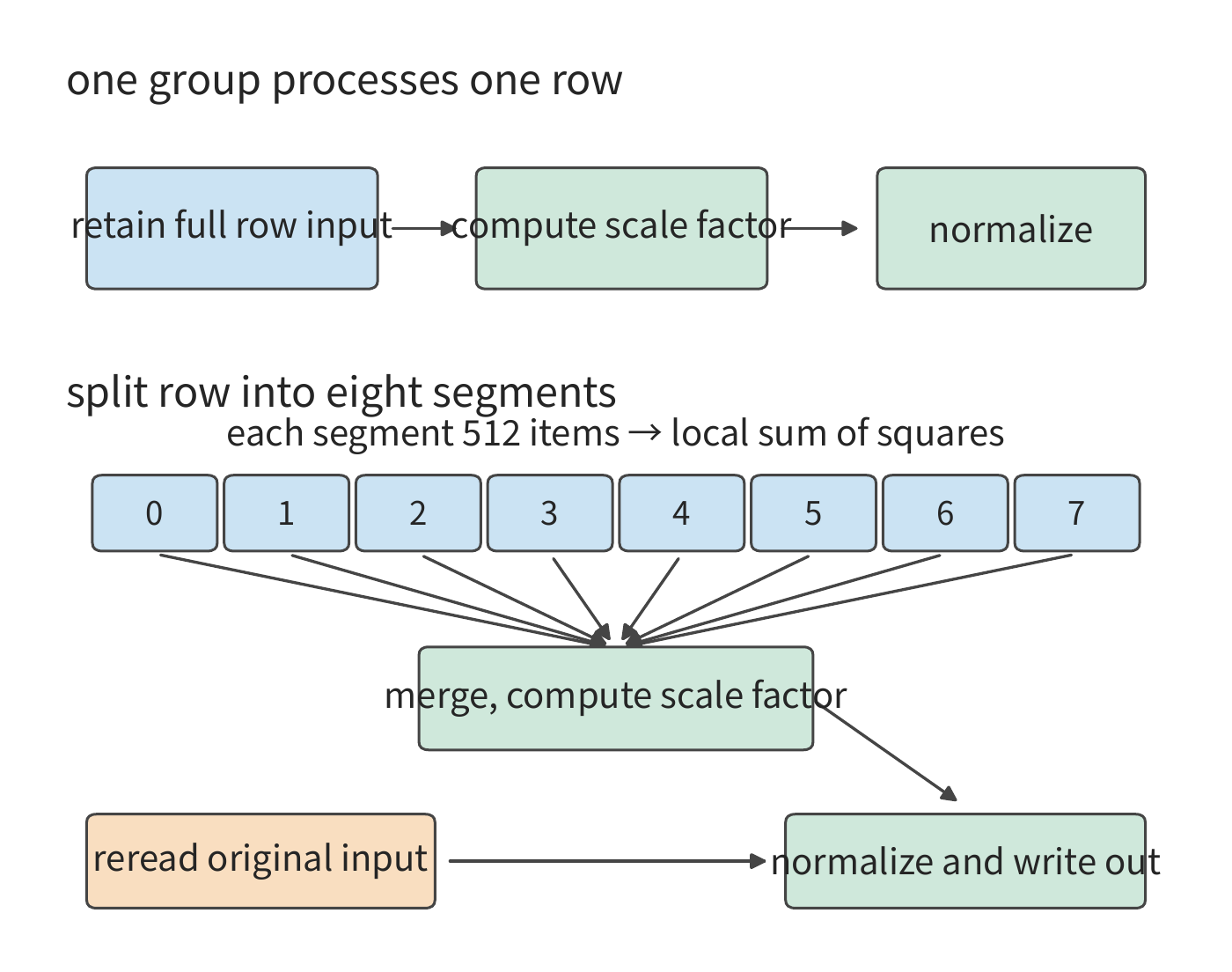
Counting along the arrows in Figure 5-11 gives the memory access cost of increasing parallel tasks. Still taking 1024 tokens, with each token's feature vector occupying one row of the input matrix. The first-stage parallel task count grows from 1024 groups to 8192 groups; 8192 FP32 local sums occupy 32 KiB, and 1024 FP32 scale factors occupy 4 KiB. A program with one group per row keeps the input resident locally, reading 8 MiB of input, rereading a BF16 gamma per row totaling 8 MiB, and finally writing out 8 MiB of result, for a total access volume of \(8+8+8=24\) MiB. After splitting, the final normalization stage rereads 8 MiB of input; the write and read of local sums and scale factors add roughly another 0.1 MiB, for a total of 32.1 MiB, and the kernel launch count rises from one to three.⁴

In the figure, each group processes only one-eighth of a row, which brings another benefit: less temporary data needs to be held. Saving a full row in FP32 requires 16 KiB, while saving one-eighth of it requires only 2 KiB. Temporary data that originally had to spill to more distant storage due to insufficient registers can now stay in registers. The benefit of splitting the reduction comes from two sources: more parallel tasks, and less temporary data per group; the cost is an extra pass over the input, plus the need to pass data between stages.

RMSNorm's split is along the reduction dimension: a row's sum of squares is split into eight local sums, which then must be merged once more. Matrix multiplication offers the same choice. For \(C_{M\times N}=A_{M\times K}W_{K\times N}\), work can be split across any of the three dimensions among different executors. Figure 5-12 shows what input each of the three splits needs and what result it produces.

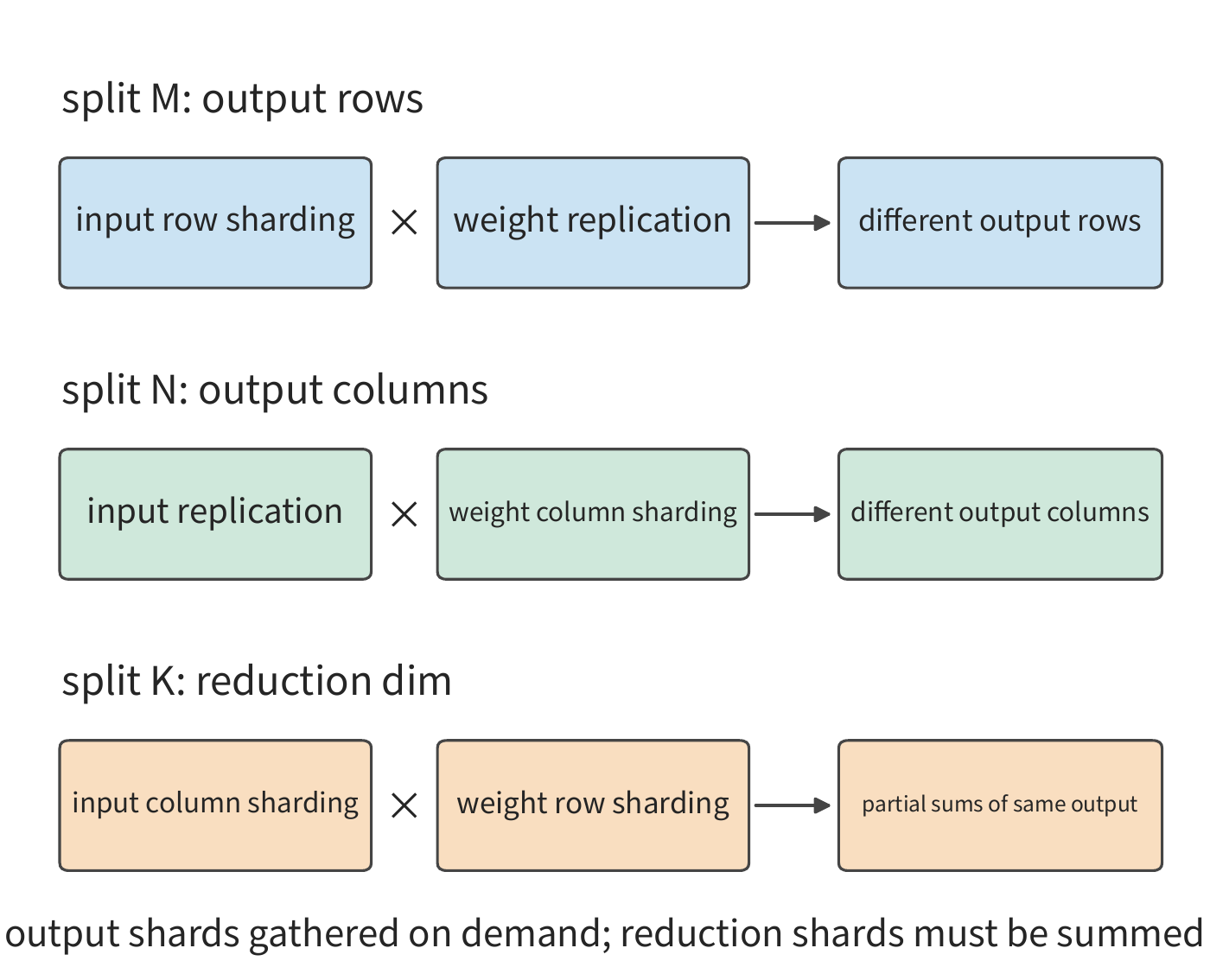
The first two splits only require inputs to be copied or sharded as needed, and the output can remain sharded until a later operator needs the complete data; the third split saves on copying input, but, like RMSNorm's local sums, adds an extra merge step. The output tile of Section 5.2.2 splits along both \(M\) and \(N\) simultaneously, then accumulates block by block along \(K\): the accumulator stays within one thread block, so merging partial sums crosses no boundary at all.

Merge order also changes the result. Floating-point addition doesn't satisfy associativity: computing \(1+2^{-24}+2^{-24}\) in FP32, adding the first two terms first leaves the sum at 1, and adding the third term still leaves it at 1; adding the last two terms first gives \(2^{-23}\), which added to 1 gives \(1+2^{-23}\). The two orders differ by one ULP (unit in the last place, the spacing between adjacent floating-point numbers at a given exponent). Bits lost in one rounding can't be recovered, and every subsequent addition continues from an already-rounded number.

This section's RMSNorm can quantify how large this difference is. Take a row of 4096 BF16 elements, where each element's square is exactly representable in FP32, so the differences among the approaches below come only from addition order. The top half of Figure 5-13 compares sums of squares computed with six different splits — 1, 2, 4, 8, 16, 32 segments — with the horizontal axis showing their distance from the exact value. When one group processes a whole row, the accumulator grows step by step to around 2038, while each term added in is only about 0.5, so the low bits keep getting rounded away, ending up 175.2 ULP below the exact value. After splitting into eight segments, each accumulator grows only to around 255, and the eight local sums are added together just once at the end, giving a result only 9.2 ULP from the exact value. The two paths differ by 166 ULP, a relative difference of about \(9.9\times10^{-6}\). So splitting changes not just the parallel task count, but precision as well.

The bottom half fixes these eight local sums and varies only the merge order. The 40,320 possible orders yield only three distinct FP32 results, differing from each other by one ULP. If an atomic add accumulates the local sums into the same address, the arrival order is determined by scheduling; running the same input through the same program twice can then yield different results. Instead, writing the eight local sums into a buffer, waiting until all of them are written, and then having one executor add them in a fixed order always gives the same result. This costs two things: an extra write-out and read-back; and the merge has to wait for the slowest segment to finish before it can start, whereas an atomic add accumulates in arrival order without waiting for all of them to be ready.

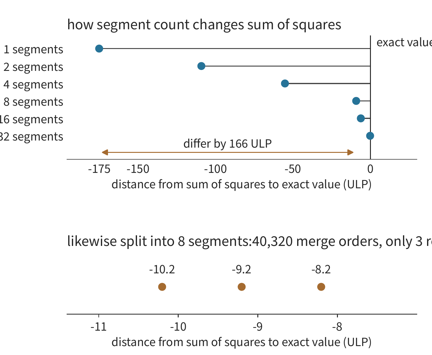
The difference doesn't stop at the sum of squares. Continuing the computation with Qwen3-8B's rms_norm_eps, the two paths' scale factors differ by 59 ULP, and the row's first output element differs by 50 ULP, and this propagates together into the next layer.³

The choice of split is therefore not just a matter of speed. As noted at the start of this subsection, how many segments to split into depends on how many parallel tasks can be arranged: with 1024 rows, one group per row is already enough; with only one row in decode, splitting is required. The same kernel will then vary its segment count with batch size, so the same row of input produces different output under different batch sizes. To make the output depend only on the input, both the segment count and the merge order must stay fixed regardless of batch size, at the cost of losing the extra parallelism gained from splitting when the batch is small. Section 10.5.3 uses exactly this point to explain why generation and training load the same weights, yet the logprob computed from the same prefix can still differ.

Tiling can also cross the boundary of a single card. Within one card, the computation of these tiles is handled cooperatively by thread blocks, shared memory, and local reductions; once split across multiple cards, executors splitting along an output dimension each have to obtain their own inputs, and executors splitting along the reduction dimension have to send partial sums to be added together — all of this movement crosses the inter-card interconnect. The mathematical dependency hasn't changed; what changes is the distance and cost of moving the data.

Scheduling, in turn, is what decides execution order, placement, buffering, and overlap after tiling. For example, after splitting along \(K\), whether to wait for all inputs to arrive before computing, or to accumulate as data arrives, changes storage occupancy and actual wait time. Samples, sequences, features, layers, and experts in a model offer further directions for division of labor; among these, layers are sequential stages in the computation graph, while experts are branches selected by routing. Section 6.1.4 will map these directions of division of labor onto the three splits here, and Section 6.2 will then derive the communication for each in turn.

Matrix tiling, bank padding, and reduction splitting are all ways of rearranging the same batch of mathematical work. Tiling lets multiple outputs reuse input, padding spreads read requests across different banks, and splitting the reduction increases the number of tasks that can run in parallel. When analyzing a program, one needs to work out precisely both the benefit and the cost of each change, and also check whether it alters the floating-point result. The companion experiments' comparison between contiguous access and wide-row reduction provide the corresponding execution records.⁵

5.3 Fusion, buffering, and pipelined execution across adjacent operators

Within a single operator, local storage can be used to reuse input. The same opportunity exists between adjacent operators: the output of one operator often immediately becomes the input to the next. If the next operator can read the result directly out of local storage, it can skip a write-back and reread. To do this, we need to determine which data the next operator will use, and when all of that data is ready.

5.3.1 Intermediate tensors and fusion boundaries

Now extend the running example to the FFN's two projections. Let \(G=XW_g\), \(U=XW_u\), with the activation chain computing \(Z=\operatorname{SiLU}(G)\odot U\), which is then handed to the down projection to bring the result back down to the hidden width. G, U, and Z all have shape \([1024,12288]\), and each occupies 24 MiB stored in BF16.

Both SiLU and \(\odot\) are elementwise operations. Z[i,j] depends only on G[i,j] and U[i,j], with no reduction across positions. So once the two elements at the same position are read in, the final result at that position can be computed directly, without first computing the whole SiLU result.

First, compare where the intermediate result \(T=\operatorname{SiLU}(G)\) goes. When executed separately, the complete T has to be written to the next storage level and then read back by the multiplication; when fused, a small piece of the SiLU result can be handed directly to the multiplication within the same kernel, freeing the local space once used. This is like handing freshly processed material on the workbench directly to the next step, skipping the round trip of sending it back and fetching it again. Correspondingly here, what's skipped is the write-back and reread of the intermediate result; both operations still have to be completed.

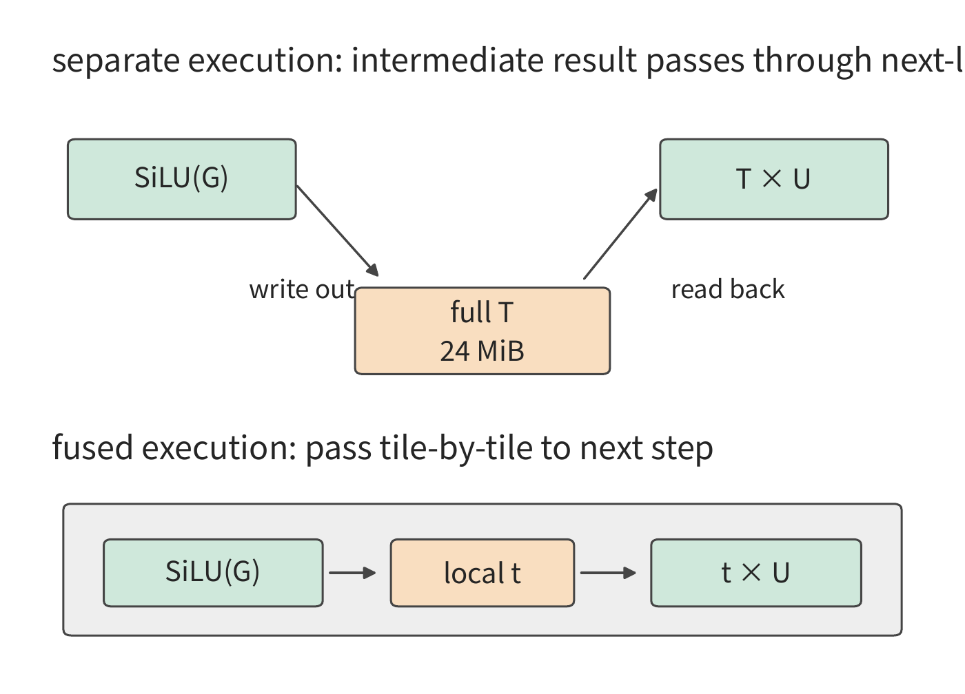
Example 5-4: How much does fusing activation operators reduce intermediate tensor read/write? Executed separately, first compute \(T=\operatorname{SiLU}(G)\), reading G and writing T, totaling 48 MiB; then compute \(Z=T\odot U\), reading T and U and writing Z, totaling 72 MiB. Total read/write volume is 120 MiB. Fusing the two steps, each time read a slice of G and U, complete SiLU and the multiplication locally, and write out Z, requiring only 72 MiB.

The 48 MiB saved is exactly one write and one read of T. Following the previous section's bandwidth model, assuming both programs have the same effective bandwidth, the time ratio is \(72/120=0.6\), a speedup of about 1.7×. The measured activation chain drops from about 14.2 μs to 7.7 μs, a measured speedup of about 1.8×. Both the theoretical calculation and the measured result point to the same source of benefit: skipping the write-back and reread of the complete T.⁷

Next, quantize Z with a fixed scale, so each element occupies only 1 byte. Converting independently requires reading the 24 MiB Z and writing out 12 MiB of quantized result, an added 36 MiB. The total for all three steps fully separate is 156 MiB; fusing the first two steps gives 108 MiB; fusing all three gives \(24+24+12=60\) MiB. Figure 5-15 draws the required input/output read/write on the left side of each bar, then adds the reads/writes of the two intermediate quantities in turn.

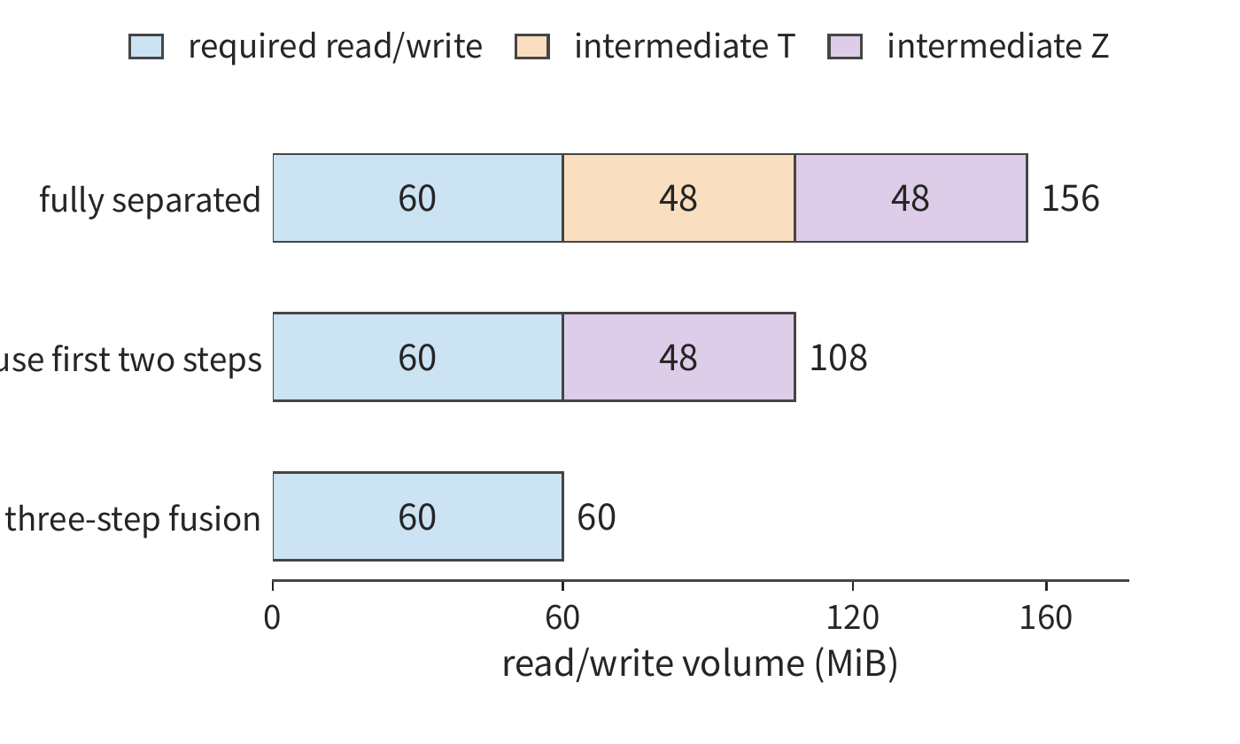
The capacity and access volume of intermediate tensors are two different things here. Suppose each step allocates its output first, then frees the input once it's no longer needed. Running SiLU independently, G, U, and T occupy memory simultaneously, with a peak of 72 MiB; fusing all three steps, G, U, and the final output occupy memory simultaneously, with a peak of 60 MiB. Read/write drops by 96 MiB, but the peak drops by only 12 MiB, because the same block of storage space can be read and written repeatedly.⁶

Since each output of an elementwise operation depends only on the input at the corresponding position, computation can happen immediately after reading, reducing how much of the intermediate result needs to be retained. For this reuse to happen smoothly, the two steps also need to use mutually compatible data layouts, and the buffer must not be overwritten before its last read completes. Below, we follow the lifecycle of one data block to analyze these two conditions.

5.3.2 Layout Transformation, Buffer Reuse, and Double Buffering

Adjacent operators sometimes use different layouts. The earlier operator may naturally write out row by row, while the later operator needs to read in a different block order. Building a separate 24 MiB reordered copy means reading the original result and writing the new one — 48 MiB in total. Alternatively, the earlier operator can write directly in the layout that the following computation needs, eliminating the separate reordering step. Comparing the total time of "compute then reorder" against "compute while writing directly in the new layout" tells us which approach is faster.

Buffering also determines whether two stages can overlap. Suppose a mover places block 0 into slot A, and the compute unit then reads A. While the compute unit reads A, the mover places block 1 into slot B; once computation moves to B, block 2 can be loaded into A. With the two slots alternating this way, the mover can write the next block while the compute unit reads the current one.

Note that "the data has finished moving" and "the data has finished being used" for slot A are two different moments. Computation begins reading only after the move finishes; only after the last read finishes can the next block be written into slot A, overwriting the previous contents. Reusing the H100 single-SM figures from Section 5.1.5: each block takes 1.29 μs to move and 0.28 μs to compute, with the mover and compute unit operating independently. Figure 5-16 shows the state of each slot across three time windows, and Figure 5-17 draws the complete movement and computation timeline based on this.

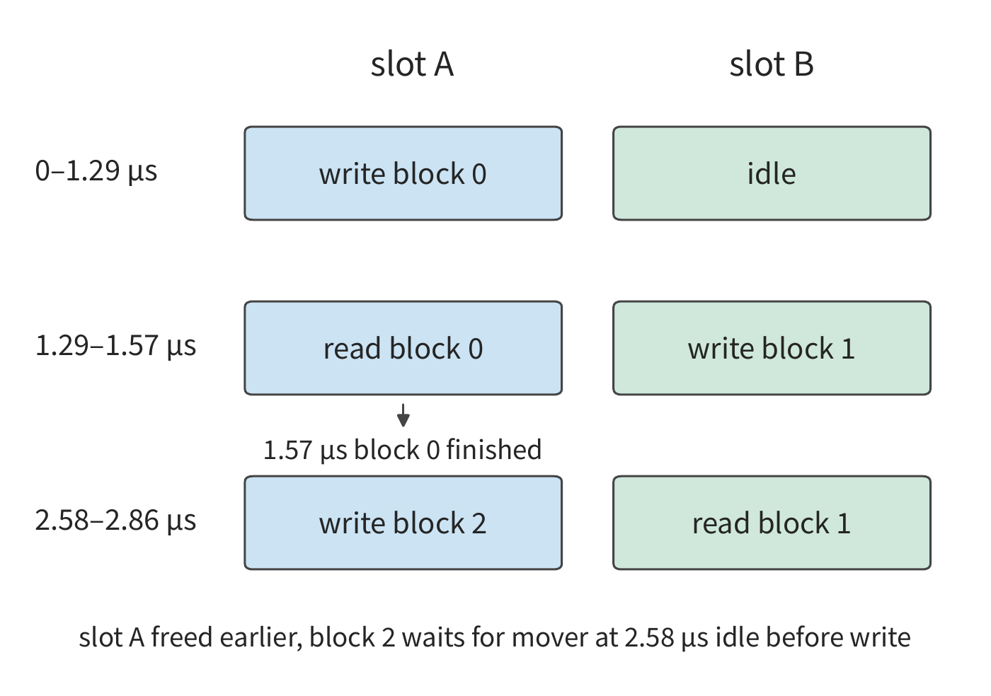
Example 5-5: How does double buffering overlap data movement with computation? Each block takes 1.29 μs to move and 0.28 μs to compute. The mover and compute unit operate independently, and we treat event overhead as zero. Executing four blocks serially takes \(4\times(1.29+0.28)\approx6.28\) μs.

With two slots, block 0 moves in during 0–1.29 μs, and computes during 1.29–1.57 μs; block 1 moves in simultaneously during 1.29–2.58 μs. Block 0 finishes computing at 1.57 μs, and slot A frees up immediately, but the mover cannot finish moving block 1 and start writing block 2 until 2.58 μs. After that the mover works continuously, delivering one block every 1.29 μs, while the compute unit stays busy for only 0.28 μs each time. The fourth block finishes at 5.44 μs — only about a 13% reduction in time.

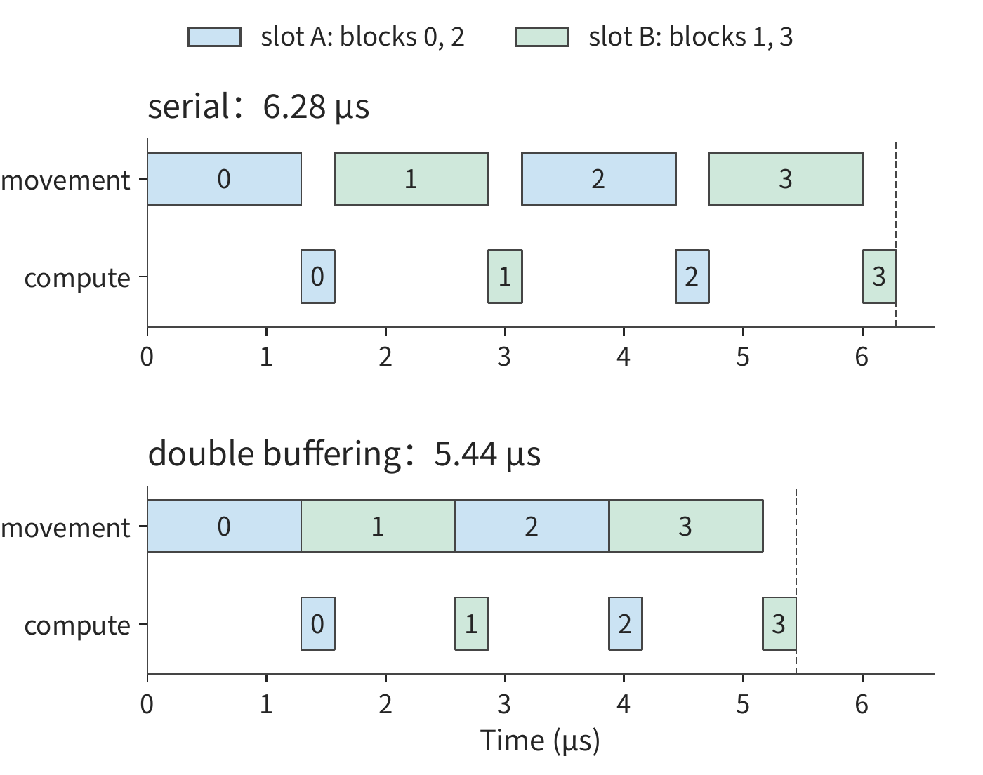
Generalizing from four blocks to n blocks: the first block must move first, then one block finishes every interval equal to the slower stage's time, and the last block still needs its computation to finish. So:

\[ T_{\mathrm{pipe}}=t_m+(n-1)\max(t_m,t_c)+t_c. \]

Here \(t_m\) is the movement time per block and \(t_c\) is the compute time per block. In the example just given, \(t_m>t_c\), the mover stays continuously busy from 0 to 5.16 μs, and the total time is \(4\times1.29+0.28\approx5.44\) μs — the compute unit is busy only about 20% of the time. Adding a third slot doesn't help: two slots already keep the mover free of idle time, so more slots cannot speed up the movement, and speeding up computation is equally useless. Two slots are the minimum configuration that allows overlap; extending the slot count to \(n\), letting movement begin \(n-1\) blocks ahead, is called \(n\) stages in CUTLASS. In this example, the mover is already working continuously, so additional stages only consume more capacity; only when the movement time per block is unstable, or when a single move's latency exceeds one block's compute time, can extra stages fill the gap — and the capacity required grows proportionally with the number of stages. To shorten the time further, the only options are to reduce the bytes moved per block — for example, by enlarging the output block as in Section 5.2.2 so each input byte participates in more multiply-adds, or by having concurrently executing thread blocks share input blocks in L2 — or to switch to a card with higher memory bandwidth.

Returning to the reordering scenario from the start of this subsection: when the two stages access data in different orders, the buffer must hold more not-yet-used data. Three queued 16 KiB blocks occupy 48 KiB, plus 32 KiB of reorder space, totaling 80 KiB. One thread block on the RTX PRO 6000 can use up to 99 KB of shared memory, which fits when resident alone; but if one SM must host two such thread blocks simultaneously, each block gets at most 49 KiB (100 KB minus 1 KiB reserved per block, split evenly). After subtracting the 32 KiB reorder space, only one 16 KiB queuing slot remains: before writing the second block, the mover must wait for the compute unit to finish using and release that slot. This mechanism — where the downstream side cannot keep up and forces the upstream side to pause — is called backpressure. Choosing a shared layout reduces queuing; enlarging the buffer allows more data that has been written but not yet used to accumulate.⁸

The host input from Section 5.1 can be organized the same way. A copy stream feeds the next batch while a compute stream processes the current one; the compute stream waits for a "copy complete" event before reading new input, and the copy stream waits for a "compute complete" event before overwriting the old buffer. These two events guarantee, respectively, that the input is ready and that the old data has been consumed; the time benefit comes from the two resources working simultaneously.

5.3.3 FlashAttention: Tiling and Online Softmax

The elementwise operations fused in Section 5.3.1 each have outputs depending only on the input at the same position; but Softmax in attention needs an entire row of scores. To compute one row of attention output, we can first turn each position's score into an unnormalized weight, use those weights to compute a weighted sum of the values, and finally divide by the sum of the weights. We can process one block at a time, recording its contribution to the weighted sum and to the total weight, then move to the next block; as long as the contributions merge correctly, there's no need to keep all the previously processed scores around. The difficulty is that Softmax takes exponentials based on the scores, and when a larger score appears later, the numerical baseline used for the accumulated results so far must be adjusted.

FlashAttention arranges storage around this block-by-block computation, reducing the memory reads and writes of the attention intermediate matrices for long sequences. The method was proposed in 2022 by Tri Dao and colleagues at Stanford University together with collaborators at the University at Buffalo, SUNY.¹⁰

Reading about FlashAttention, the author was reminded of an experience with AKG back in 2019. At the time, in order to fuse the Softmax operator, the author searched widely for a suitable online algorithm, and eventually found research published by NVIDIA in 2018, which made it possible to combine AKG's tiling and fusion capabilities to chain the preceding matrix multiplication together with the following Softmax. The author didn't even understand the attention mechanism at the time, and only later realized that this had stumbled onto one of the core ideas of FlashAttention. Getting from that step to the full FlashAttention still required folding the subsequent weighted sum with V into the same online update, and arranging on-chip storage and data movement around the complete attention computation. The derivation below shows how this seemingly local algorithmic change eliminates the large intermediate matrices.

Back to the attention computation itself. Standard attention first computes \(S=QK^\mathsf{T}/\sqrt d\), then computes \(P=\operatorname{softmax}(S)\), and finally computes \(O=PV\).

Handing these three operations to separate general-purpose operators lets us compose the program directly following the formula, with operators exchanging results through intermediate tensors. Once we understand the full data dependencies of the attention computation, we can adopt a different compilation and execution strategy: exploit the reduction structure of Softmax to cross the boundaries of independent operators and compute continuously on small blocks of data. Below we first calculate the cost of fully preserving the intermediate tensors as originally done, then derive the state that must be kept for block-by-block computation.

Take one head, with sequence length \(L=8192\) and head dimension \(d=128\), computing attention over all tokens. Q, K, V, O use BF16 and occupy 2 MiB each; the complete S and P use FP32 and occupy 256 MiB each. Q, K, V are each read once and O is written once, totaling 8 MiB; S and P are each written once and read once, yet this transfers 1 GiB of data. The intermediate matrices grow with the square of the sequence length, causing this large volume of reads and writes.⁹

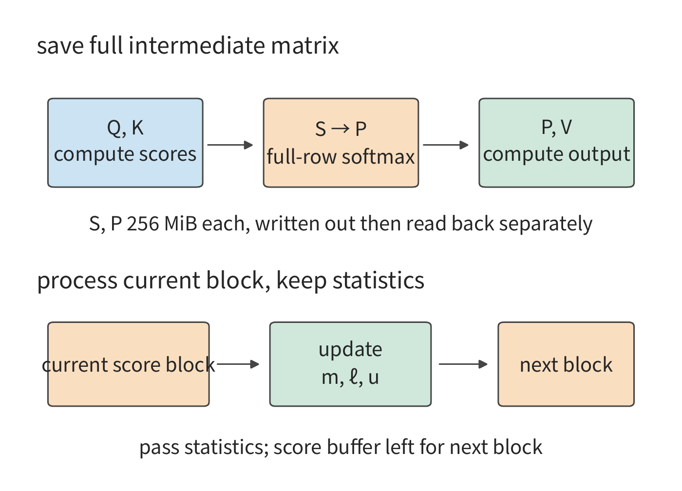
To eliminate this 1 GiB of intermediate reads and writes, we might follow the approach in Section 5.3.1; but directly applying elementwise fusion runs into an obstacle: Softmax's denominator is the sum of exponentials over the entire row. Having read only the previous block, we don't yet know the final denominator, nor whether a larger score will appear later.

To discard scores already processed, we need to retain three quantities: the running maximum score m, the exponential sum \(\ell\) relative to m, and the weighted sum of values u under the same exponential weighting. Here u is usually a vector; we'll first work through the update process with a small scalar example.

Example 5-6: How does online Softmax merge block results while keeping normalization correct? The scores are \([0,\ln2]\), with corresponding values \([1,3]\), and each block contains only one element. The first block gives \(m=0,\ell=1,u=1\). After processing the second block, the maximum rises to \(\ln2\), so we multiply the original \(\ell\) and u by \(r=1/2\); the new element's exponential is 1, so \(\ell'=1/2+1=1.5\), \(u'=1/2+3=3.5\), giving a result of \(7/3\). Processing the whole row at once, the two weights are proportional to 1 and 2, giving the same result of \((1+2\times3)/3=7/3\).

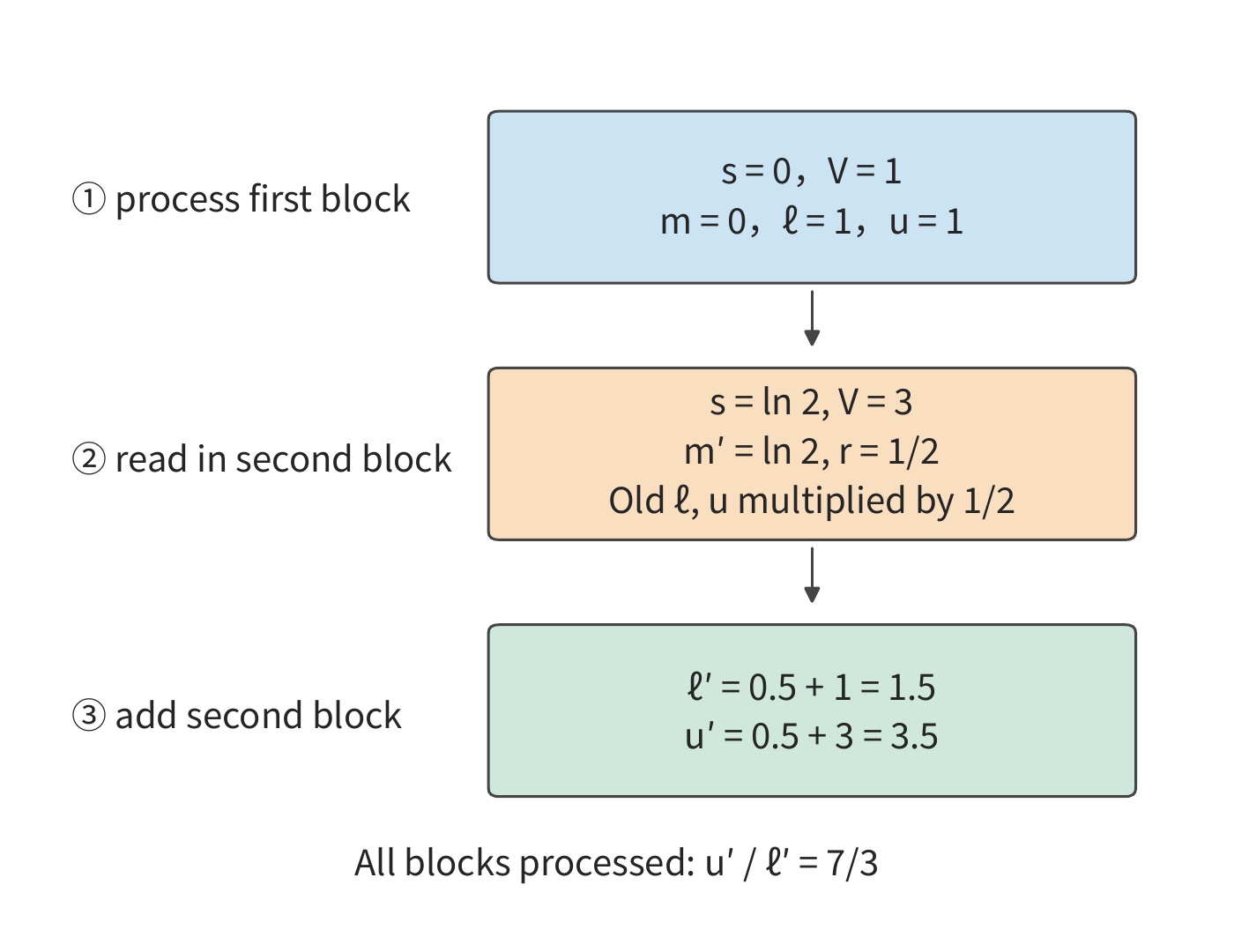
In the small example, the second block raises the maximum from 0 to ln 2. The old term's exponent was originally 1, and shifting to the new baseline turns it into 1/2; the old contribution in the denominator and the old contribution in the numerator must be scaled down together to keep their relative weight unchanged.

Generalizing to a full row of scores, subtracting the shared maximum avoids exponential overflow. Let \(\ell=\sum_j\exp(s_j-m)\), \(u=\sum_j\exp(s_j-m)V_j\), with the final output being \(u/\ell\). When a new block arrives, shift the old state to the new maximum baseline, then add the new block's contribution:

\[ m'=\max(m,\max(s)),\qquad r=\exp(m-m'),\qquad p_j=\exp(s_j-m'), \]

\[ \ell'=r\ell+\sum_jp_j,\qquad u'=ru+\sum_jp_jV_j. \]

The sum on the right only ranges over j in the new block — all the old blocks' contributions are already captured in \(\ell\) and u, with no need to read the old scores back.

FlashAttention exploits exactly this recurrence relation to eliminate storing the full S and P. After each block is processed, m, \(\ell\), and u are updated; that block's scores and probabilities can be discarded once used, and their buffer can be handed to the next block. Within the same attention scope, the matching between queries and keys and the weighting of values still all have to be computed; what changes is the order of computation and how intermediate results are kept, and floating-point execution also introduces rounding differences.

This turns the problem of storing the complete score matrix into the problem of arranging the current block within fast storage. Next we determine how many rows of Q and how many rows of K/V to process at once, in order to make the best use of this space. Take the 99 KB of shared memory (101,376 bytes) available to one thread block on the RTX PRO 6000 as the fast buffer, keeping a rows of Q and an FP32 output accumulator at once, with a score block of size a×b. K and V reuse the same b×d input slot across stages, scores and probabilities reuse one a×b slot, and three FP32 vectors are set aside for per-row statistics and update staging. The local storage requirement is:

\[ S=\underbrace{2ad}_{Q}+\underbrace{2bd}_{K/V\text{ slot}}+\underbrace{4ab}_{\text{scores/probabilities}}+\underbrace{4ad}_{\text{output accumulator}}+\underbrace{12a}_{\text{per-row state}}\le101376. \]

The smaller the K/V block, the less space it and its score block consume, allowing more Q rows to fit. More Q rows sharing a single K/V pass means the full K/V gets re-read fewer times. Taking b=64 fits a=82 rows of Q, requiring \(\lceil8192/82\rceil=100\) complete passes. Each pass reads 4 MiB of K/V, plus one Q read and one O write-back, totaling \(100\times4+4=404\) MiB.

Shrinking b to 1 fits a=128 rows of Q, dropping the number of passes to 64, with access volume falling to \(64\times4+4=260\) MiB. But each pass now goes from 128 K/V blocks to 8192 blocks, and the online state must be updated far more frequently.

K/V block rows b	Q rows fit a	full K/V passes	buffer-to-next-level traffic	Q block–K/V block state updates
1	128	64	260 MiB	524288
64	82	100	404 MiB	12800
128	53	155	624 MiB	9920

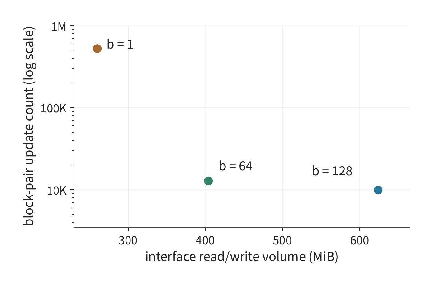
Figure 5-20 puts both costs on the same plane: further left means less data read, further down means fewer updates performed. Shrinking from a 64-row block to a 1-row block reads 144 MiB less, but raises state updates from 12800 to 524288 — about 41 times as many. Each update must execute loop control, a maximum comparison, and exponential and output scaling; processing only one row of K/V at a time also makes one dimension of the matrix multiply too small to make good use of the matrix compute unit. Smaller K/V blocks reduce reads but increase the number of updates; larger blocks favor the matrix compute unit and reduce loop overhead. Choosing a block size therefore requires weighing both kinds of cost together.

Online reduction eliminates the reads and writes of the complete intermediate matrices, but the within-block matrix multiply, exponential computation, and statistic updates still have to run. Later optimizations turn to this remaining work. FlashAttention-2 improved the division of tasks among threads, reducing intermediate data exchange and non-matrix operations; FlashAttention-3 uses asynchronous execution so that movement, matrix multiplication, and Softmax overlap with each other. Having eliminated the huge intermediate matrices, these improvements further shorten the remaining computation and movement time.¹⁰

To examine the effect of these mechanisms in an actual program, an accompanying experiment compared two implementations behind the same attention interface in PyTorch. Here, backend refers to the computation program the framework actually selects internally for the interface: given the same Q, K, V, the framework can complete the attention computation with different programs.

The math backend (SDPBackend.MATH) composes general-purpose operations such as matrix multiplication and Softmax following the attention formula, keeping the complete score and probability intermediate matrices. The FlashAttention backend (SDPBackend.FLASH_ATTENTION) uses the tiling and online-reduction method described above, avoiding storage of the complete intermediate matrices. The experiment specified each of these two backends in turn and compared the time and additional GPU memory needed to complete the same attention computation.

The experiment used an RTX PRO 6000 Blackwell, with BF16 input and output, processing one sequence and one attention head at a time, with head dimension 128. The sequence length was 8192 tokens; causal attention was used, meaning each position only attends to itself and earlier positions. After warmup, a CUDA Graph was used to pre-record and repeatedly replay a set of GPU operations, to avoid interference from per-call host submission. Measured per attention computation, the math implementation that keeps the complete intermediate matrices took about 2.6 ms, while the FlashAttention implementation using tiling and online reduction took about 80 μs — a speedup of about 33 times.¹¹

We also compared the peak additional GPU memory used by a single ordinary call. With input Q, K, V already resident in GPU memory, the measurement covers the output and temporary workspace: about 848 MiB for the math implementation, versus about 22 MiB for the FlashAttention implementation.

This side-by-side comparison of the two full implementations shows how tiling, online reduction, and fusion work together: tiling lets the current data fit in fast storage, online reduction lets Softmax be computed block by block, and fusion eliminates the write-back of within-block intermediate results. Together, the three change both the execution time and the intermediate storage requirements.

5.4 Compilers: Representation, Transformation, and Selection

The previous two sections chose loops, block sizes, buffers, and operator boundaries through manual analysis. Real models use many input shapes and operator combinations, and each accelerator has a different memory hierarchy and set of execution resources. The compiler's job is to represent these implementation choices as programs, rule out incorrect transformations based on dependencies, and then compare the execution cost of the remaining implementations.

5.4.1 Why Compare Multiple Implementations

Revisit the elementwise chain: SiLU applies a nonlinear transformation to each number, which is then multiplied elementwise with another input, and finally quantized to a low-bit representation. Between each pair of adjacent operators, we can choose to execute them separately or fused, giving four partitions: all three steps separate, the first two fused, the last two fused, or all three fused. If a chain contains ten operators, there are \(2^9=512\) ways to partition the adjacent boundaries. Each partition can also choose its own block size, local layout, and pipeline depth.

These choices interact with each other. Merging two steps eliminates an intermediate write-back, but also increases the amount of data that must be kept live at once; more temporary data then changes which block sizes are feasible. The compiler therefore must represent computation content, execution order, and data placement all at once. Recording only an operator name gives no way to derive these costs.

A compiler can choose an implementation in three steps. First, express the mathematical operation as loops and array accesses, making explicit which loops can be transformed and what their read/write relationships are. Second, check legality against the read/write dependencies and numerical rules. Third, combine capacity constraints and measured timing to compare execution cost. Below, readable loop code demonstrates the first two steps, followed by an explanation of how the automatic operator code generation system AKG organizes the whole process through polyhedral compilation (a compilation method that describes loop iterations and array accesses using linear constraints).

5.4.2 Expressing Tiling and Fusion with Loop Transformations

Section 5.2 determined how much data to process per block; we still need to decide the order in which these blocks are computed. Even with the same data sliced the same way, if a piece is swapped out right after use and then has to be moved back in later, unnecessary accesses still occur. Loop transformations let a program express these arrangements: split breaks a loop into "which block" and "which position within the block"; reorder adjusts the traversal order so that data about to be reused has a chance to stay in local storage. Choosing at which loop level to keep or use an intermediate result then makes explicit how long it must be retained.

Take \(Y=\operatorname{SiLU}(AW)\), using \(M=1024,K=4096,N=12288\) as before, with the matrix multiply accumulating in FP32 and the result rounded to BF16 before the activation. The most direct program first generates the complete C, then iterates over C to generate Y:

for i in range(M):
    for j in range(N):
        acc = 0.0
        for k in range(K):
            acc += A[i, k] * W[k, j]
        C[i, j] = round_to_bf16(acc)

for i in range(M):
    for j in range(N):
        Y[i, j] = silu(C[i, j])

The first transformation is split. Split i into a block index \(i_o\) and an in-block coordinate \(i_i\), with \(i=64i_o+i_i\). The original 1024 rows now become 16 blocks of 64 rows each. Doing the same for j gives 192 column blocks. Splitting both output dimensions together forms 64×64 tiles.

Splitting first changes how the indices are represented. To finish one tile continuously, we also need reorder: iterating over output blocks in the outer loop, and over the elements within a block in the inner loop. Then split K into 128 reduction blocks of 32 each. The program picks one output tile, loads the needed A, W piece by piece, and accumulates into that same output block.

With this loop structure in place, we can now determine how long the input blocks must be kept. The current blocks of A and W each occupy 4 KiB, and can be replaced right after one reduction block's computation; the 4096 FP32 accumulators occupy 16 KiB, and must be kept until all 128 reduction blocks have finished. These two kinds of buffers therefore should be allocated and released at different loop levels.

Finally, adjust the compute location of the activation. Once one output tile has finished all its K reductions, its 4096 C values are all computed, and SiLU can be applied and Y written out immediately — this doesn't affect the fact that other output tiles haven't finished yet. This way, only the current output block's result needs to be kept locally; the full 24 MiB of C is no longer needed, eliminating the 48 MiB of write-back and re-read.

for io in range(ceil_div(M, BM)):
    for jo in range(ceil_div(N, BN)):
        acc = zeros_fp32(BM, BN)
        for ko in range(ceil_div(K, BK)):
            a = load_tile(A, io, ko, BM, BK)
            w = load_tile(W, ko, jo, BK, BN)
            matmul_accumulate(acc, a, w)
        c = round_to_bf16(acc)
        store_tile(Y, io, jo, silu(c))

Here load_tile and matmul_accumulate represent block loading and matrix accumulation respectively; the last, incomplete tile is masked to mark the valid positions. The indentation in the pseudocode clearly marks these before-and-after relationships: input blocks are updated inside the ko loop, the accumulator persists throughout the entire ko loop, and the activation computation happens after the ko loop finishes.

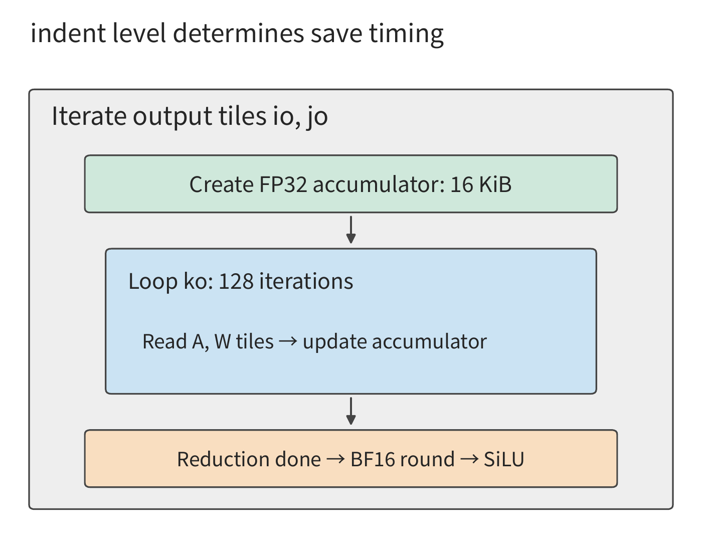
These scheduling actions have counterparts in programming systems. Halide is a programming system that separates "what to compute" from "how to schedule," letting programmers use actions like split, tile, and reorder to change how execution proceeds. Here we call the operator producing an intermediate result the producer, and the operator that consumes that result the consumer. compute_at specifies at which loop level of the consumer the producer executes. TVM is a compilation system for tensor computation that likewise uses schedules to specify compute location and cache read/write, letting adjacent operators compute continuously on the same piece of data.¹⁴

Compute location simultaneously determines reuse versus recomputation. Placing the computation that generates an intermediate result at the outermost level computes the complete result up front, available for all subsequent computations to read; placing it inside a later computation's block loop computes only the portion currently needed. If multiple output blocks need the same portion of an intermediate result, computing it within each block causes duplication. The compiler must therefore compare two approaches: keeping the intermediate result for multiple reads, or recomputing it before each use.

fuse in a loop can also merge multiple iteration dimensions into one. For example, the two-dimensional coordinates of the 16×192 output blocks can be converted into a single linear index from 0 to 3071, then distributed among the accelerator's work groups. This changes how output blocks are traversed and how tasks are assigned; placing SiLU right after the matrix multiply's tile eliminates the write-back and re-read of the intermediate matrix. Both can be combined within the same schedule.

5.4.3 How dependencies and rounding constrain transformations

The previous subsection moved activation into the output tile, but still scheduled it after the ko loop ends. Two numbers explain why. Suppose one output has two partial sums, 1 and −1; the complete sum is 0, and SiLU(0) = 0. If SiLU is applied to each partial sum before adding, the result is \(\operatorname{SiLU}(1)+\operatorname{SiLU}(-1)\approx0.4621\). Moving the activation computation before the complete summation has already changed the computation.

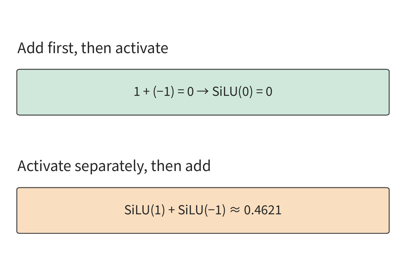
The dependencies the compiler must respect therefore have two levels: partial sums for the same output must be combined according to reduction rules, and subsequent operators must wait for the results they need. Different outputs can be computed in parallel; the reduction for a given output and its subsequent operations must execute in dependency order.

Chunked reduction is bound by this same dependency constraint. FlashAttention (Section 5.3.3) can complete computation chunk by chunk because it retains m, \(\ell\), and u, and adjusts the previously accumulated exponential sum and weighted value whenever the maximum changes. Keeping only each chunk's already-normalized output loses the relative magnitude of the denominators across chunks. For example, if two chunks each contain a single value, 1 and 3, the within-chunk outputs remain 1 and 3; from these two outputs alone, there is no way to tell whether the full-row softmax should assign them a weight ratio of 1:2 or 2:1. Chunked reduction must therefore retain enough statistics to correctly merge the results of each chunk.

Floating-point rounding further constrains the transformation. The original program rounds an FP32 accumulation result to BF16 before activation; the fused program must also execute round_to_bf16 before activation. The intermediate value can pass directly from a register to the activation, but this rounding step still occurs. Where data resides and its numerical format are two independent choices.

Example 5-7: How does a whole-row quantization scale constrain the order of chunked computation? A row contains 256 elements, split into two chunks of 128 elements each; the first elements of the two chunks are 1 and 10, respectively, with the rest zero. Quantization uses the E4M3FN format: an eight-bit floating-point representation with a sign bit, four exponent bits, and three mantissa bits, with a maximum finite value of 448. The scale is determined by the maximum absolute value across the whole row; the subsequent dot product uses a weight of 1 only for the first element. The result therefore depends entirely on how that first element is quantized.

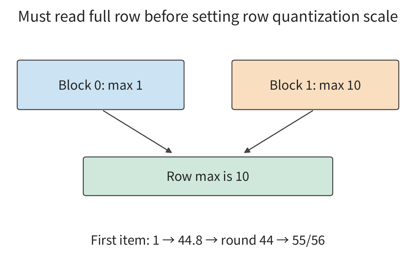
Reading the whole row first gives a maximum of 10. The first term is scaled to \(1\times448/10=44.8\), rounded to the representable value of 44 in this format, and dequantized to \(44\times10/448=55/56\). If quantization happens right after reading the first chunk, the maximum at that point is 1, so the first term can be represented exactly as 448, and the dequantized result is exactly 1.

Once the 10 in the second chunk has been read, no adjustment to the scale used in subsequent computation can undo the fact that the first term has already gone through the 44.8→44 rounding. The two approaches differ by \(1/56\), about 1.8%. Therefore, when the scale is determined from the whole row's maximum, the entire row must be read first to find that maximum, and only then should quantization proceed.¹⁵

These examples show which transformations are permissible and which computation orders must be preserved. Outputs can be executed in any order relative to each other, inputs can be cached in chunks, and computed results can be fed directly to subsequent operations; the way reductions are combined and where quantization rounding occurs, however, are part of the operation's definition and must be preserved across transformations.

5.4.4 AKG: Organizing loops and storage with polyhedral compilation

AKG is an automatic code generation and optimization system for tensor operators, whose core technique is polyhedral compilation. This method represents regular loops as three kinds of information: which iterations execute, which array elements each iteration reads and writes, and which reads and writes must preserve their relative order. Loop bounds and regular subscripts can be described with linear constraints, which is where the name "polyhedral" comes from. With this representation, the compiler can derive dependencies between iterations and adjust execution order accordingly.¹²

Take matrix multiplication as an example: the compiler can determine that different i, j pairs correspond to different outputs, while updates along k point to the same accumulated result. Once a 64×64×32 tile is chosen, the required A and W regions can also be derived from array accesses: A is 64×32, W is 32×64. This determines both the loop execution order and which data must be read in, as well as how long that data must be retained.

AKG generates a polyhedral representation from tensor expressions, combining tiling and hierarchical fusion: the outer level arranges the execution order of the whole operator, while the inner level arranges contiguous computation of each chunk and its local caching. Storage management allocates on-chip space and inserts data movement based on these regions; code generation then maps the computation onto hardware execution modes, and the tuning stage selects parameters such as tile shape. The manual process described earlier — "split the loop, determine the read region, retain the accumulated result, and apply activation after the reduction completes" — becomes, here, a set of interconnected compilation steps.

Analyzing computation and storage together also explains why fusion can increase memory access. In the earlier elementwise chain, fusion reduced reads of intermediate values by avoiding round trips; if the intermediate result instead uses a lower-bit representation and must be read repeatedly by subsequent computation, retaining it can actually reduce total reads.

Example 5-8: Does quantization executed separately or fused into the matrix multiplication produce less read/write traffic? Take a \([4096,4096]\) FP16 input A, occupying 32 MiB, which becomes 16 MiB after quantization to FP8; the FP8 weights are \([4096,1536]\), occupying 6 MiB, and the FP16 output occupies 12 MiB. The output is tiled at 128×128, giving 32 row blocks and 12 column blocks. Each output block independently reads the data it needs, and the quantization scale comes from the row's maximum value.

Consider first the approach where quantization runs separately. For each row processed, 8 KiB of local space holds that row's input, from which the scale is computed and the row is then quantized. All input is read once, totaling 32 MiB, and the quantized result is written out, totaling 16 MiB. Afterward, each of the 12 output column blocks reads the FP8 input once, totaling 192 MiB. So the input-related read/write volume is \(32+16+192=240\) MiB.

Once quantization is fused into the matrix multiplication, the original 32 MiB input is read first to compute the per-row scale; each of the 12 column blocks then reads the original 32 MiB input again and quantizes it locally. Input-related access totals \(32+12\times32=416\) MiB. Although this saves writing out the 16 MiB of quantized result, each column block's input read grows from 16 MiB to 32 MiB, and the 12 reads add 192 MiB.

Both schemes have 32 row blocks each reading 6 MiB of weights, and then writing 12 MiB of output, totaling \(32\times6+12=204\) MiB. The total access volumes are therefore \(240+204=444\) MiB and \(416+204=620\) MiB respectively — fusion increases access by about 40%.

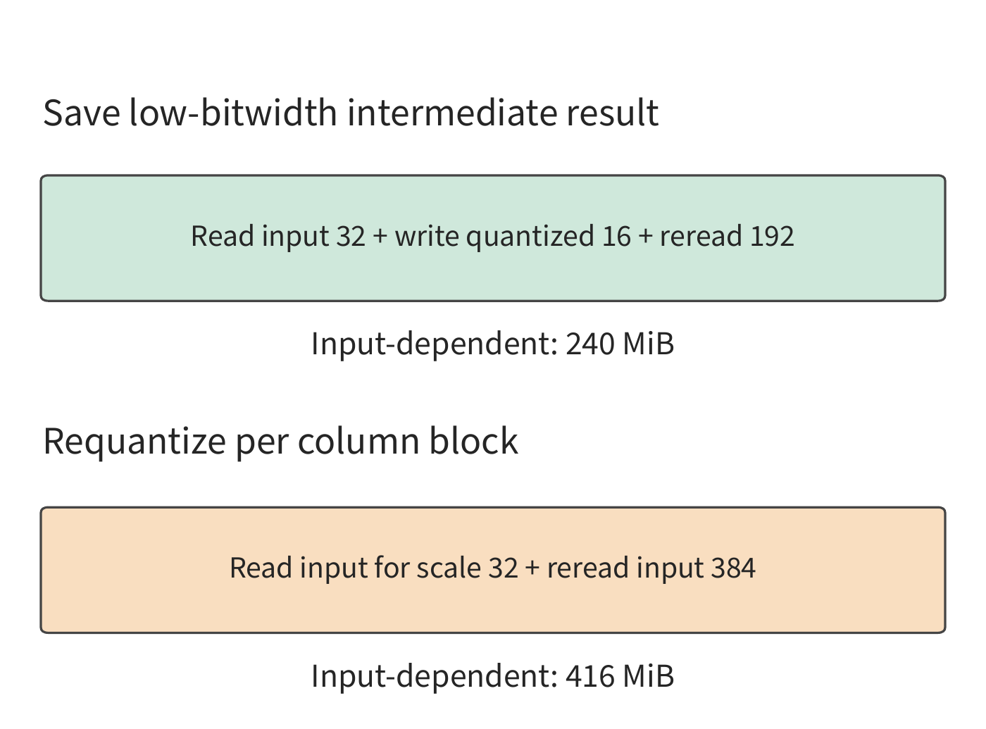
In Figure 5-24, what determines the gap is the repeated reads feeding the 12 column blocks: each read handles double the data volume. The number of output column blocks thus directly determines the difference in memory access between the two approaches. Each additional column block adds 16 MiB of reads for the scheme that retains the quantized result, and 32 MiB for the fused scheme. Putting all 1536 output columns into the same block eliminates this cross-block repetition; the corresponding output accumulator then grows from 128 columns to 1536 columns, requiring 12 times the space. So whether to fuse quantization still comes down to comparing local storage footprint against data reuse, as discussed in Section 5.2.¹⁵

AKG considers fusion and tiling together precisely to handle this kind of interaction. Once the location of intermediate-result computation changes, both which data each output block reads and how many times it reads it change; buffer requirements shift accordingly, which in turn affects the block sizes that can be used.

5.4.5 Cost estimation and empirical selection

Example 5-8 already compares two implementations by read/write volume. Facing more combinations of tiling and fusion, a compiler narrows the search the same way, step by step: first check dependencies and numerical rules, then rule out implementations that don't fit in local storage, and finally estimate execution cost to decide which implementations to test first. Section 5.2 already gave one estimation method: comparing two tiles using access volume and effective bandwidth. A compiler can also factor in matrix-instruction utilization, register requirements, and launch cost to determine the testing order among implementations.

Continuing with the matrix example and the RTX PRO 6000's shared memory from Section 5.2, the selection process can be organized into the table below. That section placed both the input buffer and the accumulator in each SM's 100 KB of shared memory; if the accumulator were instead placed in registers, shared memory and registers would need to be checked separately, as in Section 5.1.5, since the two capacities cannot borrow from each other. If both candidates were changed to double buffering, input usage would double, making the working sets 32 KiB and 96 KiB respectively, and the number of thread blocks resident per SM would change from 4 and 1 to 3 and 1.

Selection step	What to fill in for this chapter's matrix example	Basis for exclusion or comparison
Fix the target	Input shape, precision, error tolerance, call frequency	Compare the same mathematical work and the same workload
List candidates	Tile, loop order, buffer count, fusion scope	Whether the compiler and hardware support them
Check feasibility	Shared memory, registers, threads, alignment, dependencies	Compiler resource reports and correctness checks
Estimate time	Compute volume, actual read/write volume, launch and layout-transform cost	Service time of each resource and the critical path
Measure and select	Time for representative shapes, variance, and the full operator chain	Minimize workload cost while keeping close candidates

Resource reports are used first to exclude candidates that don't fit in the available capacity; the remaining candidates are then measured for effective bandwidth, compute time, and behavior across the full operator chain. If register spilling, matrix-edge padding, or reduced concurrency offsets the benefits of reuse, the process returns to the candidate table to change the block shape or buffer count. Chapter 6 follows the same process, but extends tile placement across multiple cards and translates cross-block dependencies into collective communication (communication operations in which multiple cards exchange or aggregate data according to a fixed pattern).

The measurement step can be illustrated with the matrix transpose program from the accompanying Experiment 5-5: the same program on an RTX PRO 6000 Blackwell takes about 7.9 μs with 16×16 blocks and about 2.9 μs with 32×32 blocks, a speedup of about 2.7×. Doubling each dimension of the block quadruples the number of elements inside it, and the storage layout and thread cooperation both change accordingly.¹⁷

TVM's auto-tuning searches over tiling, loop order, and other scheduling schemes based on measured hardware results; letting an agent capable of invoking compilation and testing tools modify the schedule or kernel code can also explore implementations outside the original scheduling templates. Both search methods evaluate compiled programs, filtering for correct implementations via numerical checks and then evaluating schedules by execution time. Evaluation targets the compiled program precisely because the compiler can fuse operators expressed separately in source code into a single kernel.¹⁶ The search method also has to address another question: which workload to use when evaluating these implementations.

Example 5-9: How does the call ratio between input shapes change the choice of operator implementation? Suppose an operator has two input shapes, A and B, and the original implementation takes 10 μs for either. A new implementation takes 5 μs for A and 20 μs for B: A's time is halved, B's time is doubled. If each shape occurs once, the total time rises from 20 μs to 25 μs, a 25% increase for the new implementation; if A is called 100 times and B once, the total time drops from 1010 μs to 520 μs, a speedup of about 1.9× for the new implementation.

Let p be the fraction of calls with input shape A. The original implementation's average execution time is 10 μs, and the new implementation's average execution time is:

\[ \overline T_{\mathrm{new}}=5p+20(1-p)=20-15p\quad\mathrm{\mu s}. \]

For the new implementation to have a shorter average time, we need \(20-15p<10\), i.e., \(p>2/3\). The crossover point in Figure 5-25 shows that the new implementation is faster only when A accounts for more than two-thirds of all calls.

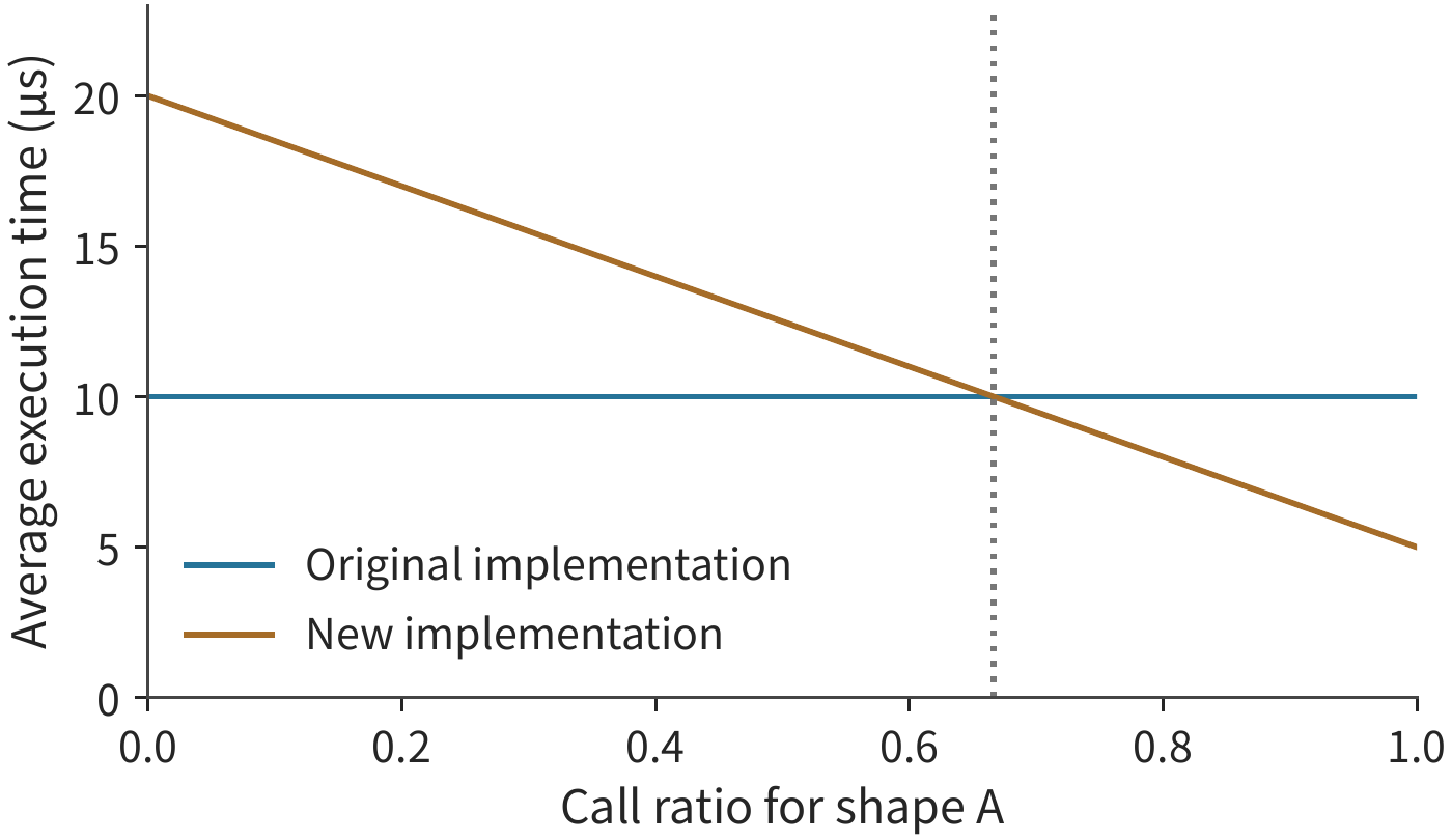
So tuning can select an implementation separately for each shape, or select a single scheme with lower overall cost based on actual call frequencies. The compilation and measurement time the search itself consumes counts as preparation cost. The accompanying agent experiment retains the code generation, repeated submission, and measurement records; the next section combines these with call counts to compute how long it takes for saved execution time to offset the search overhead.¹⁸

5.5 Runtime: submission, replay, and dynamic shape

Once the compiler selects an accelerator program, the runtime still has to repeatedly prepare inputs, select programs, submit tasks, and manage buffers. Even with the same kernel code, changing how it's submitted, or reusing existing preparation results, changes the total time. This section continues the timeline from Section 5.1, analyzing this host-side work.

5.5.1 Overlapping host preparation with accelerator computation

Section 5.1 distinguished CPU submission time from accelerator execution time, and Section 5.3 showed that the two kinds of resources can overlap. Apply both points to a single forward pass of a model: the CPU checks shapes and prepares parameters or metadata for the next stage while the GPU executes the current stage. If preparation for the next stage can happen early, the two sides form a pipeline; if the CPU waits until the GPU finishes before starting to prepare, the accelerator stalls between stages.

Example 5-10: Why does the host become the bottleneck after the accelerator speeds up? Suppose there are 100 segments of work, each requiring 20 μs of host preparation and 20 μs of accelerator computation. The data needed to prepare the next segment is already known, buffers are sufficient, and the two kinds of resources are independent. Strict serial execution takes \(100\times(20+20)=4000\) μs; with pipelining, the first segment's preparation completes first, and thereafter one segment finishes every 20 μs, giving a total time of \(20+100\times20=2020\) μs.

Shortening accelerator computation to 5 μs, the host still takes 20 μs to prepare each segment. The pipeline becomes \(100\times20+5=2005\) μs, only 15 μs less than before. The CPU's task-submission speed hasn't improved, so the faster the GPU computes, the longer it waits for the next task. Shortening host preparation time to 5 μs as well lets both sides complete a segment every 5 μs, bringing completion time down to \(5+100\times5=505\) μs.¹⁹

Figure 5-26 draws the timelines for the first four segments under all three scenarios.

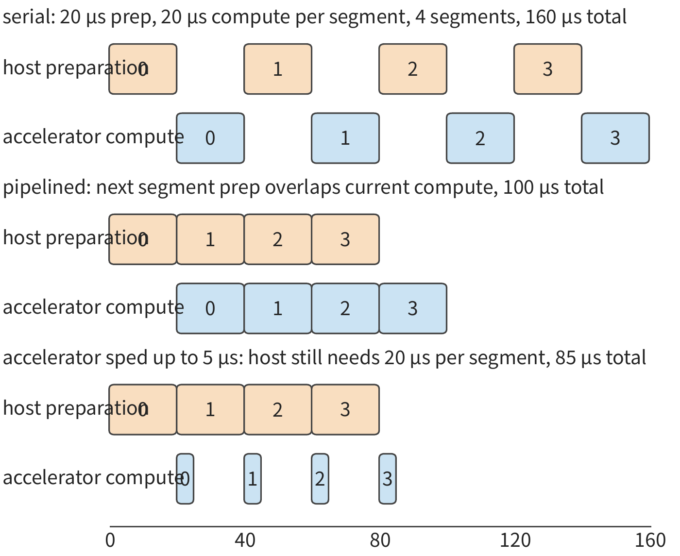
This example points to two directions for host-side optimization. One is to reduce preparation work — for example, by reusing an already-determined shape and execution plan (kernel selection, task partitioning, and workspace arrangement determined in advance based on conditions such as request length and cache layout). The other is to move preparation earlier, into the accelerator's execution window for the previous segment — for example, asynchronously processing the previous round's output. The two respectively reduce the amount of work in the pipeline and the gaps between stages.

In autoregressive generation, whether preparation can happen early depends on whether the needed data has already been computed. The next step's computation needs the token chosen in the previous round; assembling the batch, updating grammar state (which, when output format is constrained, records how far the generated content has matched the grammar), and determining whether to stop each require their own respective results. The runtime can perform work that doesn't depend on these results early, reducing the wait between rounds. The asynchronous execution and scheduling evolution in engines such as vLLM revolve around exactly this issue.²¹

Once a dedicated accelerator shortens model execution to well below the host's per-round preparation time, the lower bound on the steady-state pipeline step interval is set by host preparation. Further shortening the step interval then requires jointly optimizing dynamic batch preparation (a batch that may gain or lose requests at every step), address updates, and submission.

vLLM's v0.6.0 release in September 2024 is an instance where host overhead dominated the step interval. Profiling before the release showed that, running Llama 3 8B on a single H100, within one step the API server took 33%, scheduling took 29%, and accelerator execution took only 38%: the API server and the inference engine ran in the same Python process, and their coroutines contended for the GIL (global interpreter lock), leaving the accelerator waiting on the host. v0.6.0 moved the API server to a separate process, communicating with the engine via a message queue and avoiding GIL contention; it also introduced multi-step scheduling, executing multiple steps continuously after a single scheduling pass, avoiding repeated input preparation; and it made output processing asynchronous, overlapping it with the next step's execution. Together, these three changes raised Llama 3 8B throughput to 2.7 times that of v0.5.3, and 70B throughput to 1.8 times.²⁰ None of these changes touched any kernel, nor did they involve a hardware swap. By the criterion in Section 1.3.4, once host-side software-abstraction overhead reaches 60% of the step interval, removing that overhead is far more effective than switching to a faster accelerator.

Besides the two adjacent rounds of the same request, there is also reusable preparation work across different calls. Two calls might separately ask the model to explain code and check tests — different input content, yet passing through the same set of model layers. When length and batch size fall within a range already supported by an existing execution plan, the runtime can reuse the program, updating only the token, position indices, and state addresses; when a new shape or control path is encountered, it selects a different execution plan. Applications express change through context, and the runtime exploits stable execution structure to reduce repeated preparation. The following computes the benefit of these two forms of reuse — graph replay and shape specialization — in turn.

5.5.2 CUDA Graph: submission benefit versus input-copy overhead

In the previous subsection, the GPU sped up but was still left waiting on the host. When a model repeatedly executes similar task sequences, much of that submission work can be reused: record the accelerator tasks and their dependencies as a graph once, then resubmit it repeatedly. With CUDA Graph, the host need only issue a single graph replay each time, rather than preparing and submitting each kernel individually again. The accelerator still executes every node in the graph — what's reduced is the host's repeated work. Figure 5-27 illustrates the difference between the two submission modes using the six kernels of a single FFN.

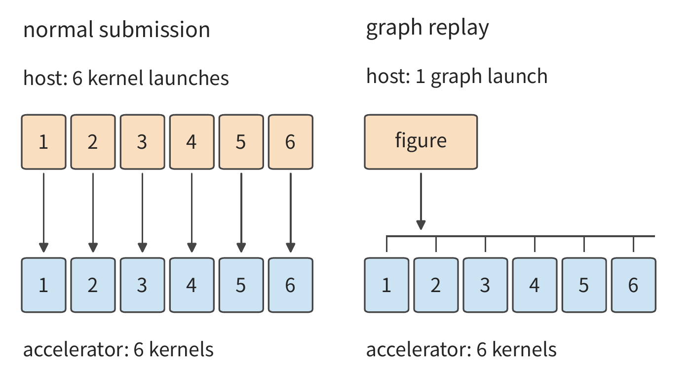
Figure 5-28 takes three FFN executions as a comparison. Ordinary submission produces 18 host kernel launches and 18 accelerator kernels; graph replay reduces this to 3 graph launches, while the accelerator still executes 18 kernels. Once the activation chain is fused, the accelerator kernel count drops to 15; adding graph replay on top, the host still needs only 3 graph launches. Fusion merges the computation of multiple operators into a single kernel, while graph replay reduces the host's work of preparing and submitting tasks one at a time.²⁵

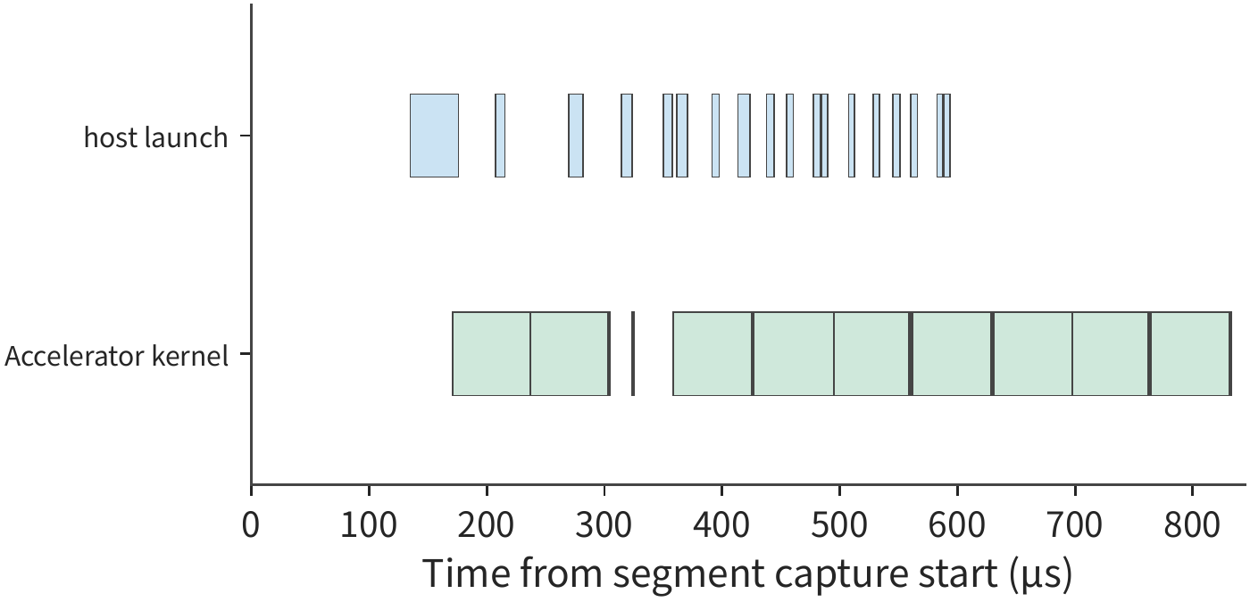
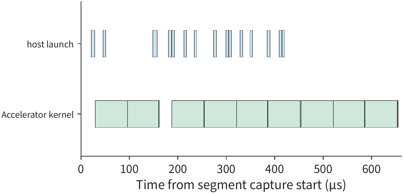
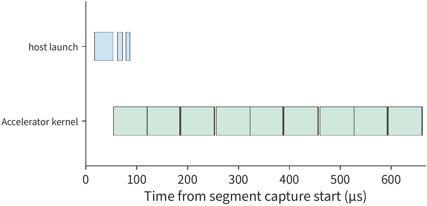
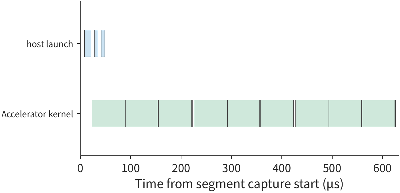
Before graph replay, new input still needs to be placed at the addresses the graph recorded. A typical implementation reserves fixed buffers for the graph; each time, the upstream writes new data into these buffers, and the graph reads from the recorded addresses. If the upstream output lives in a different tensor, an extra copy is needed before graph execution; if the upstream writes directly into the fixed buffer, this copy can be skipped.

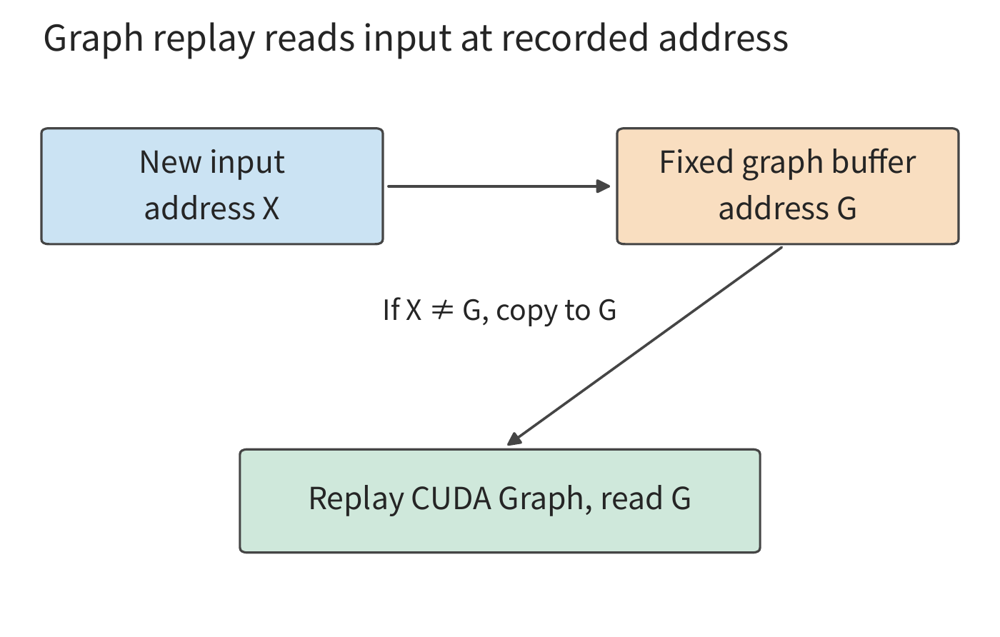
Example 5-11: When does input copying offset the benefit of graph replay? Ordinary execution takes 20 μs of accelerator computation plus 20 μs of accelerator time waiting for the host to submit tasks, totaling 40 μs. Graph replay plus metadata preparation takes 5 μs, with accelerator computation still at 20 μs. The graph would originally save 15 μs.

Take a BF16 input of \([256,4096]\) required for graph execution, with a data volume of 2 MiB. The copy both reads the source and writes the destination, for a combined read/write volume of 4 MiB; at the RTX PRO 6000's memory bandwidth of 1792 GB/s (shared between reads and writes), the copy takes about 2.3 μs, making the graph's total time about 27.3 μs — about 12.7 μs less than ordinary execution.

Keeping computation and preparation time fixed, expand the input to 2048 rows, raising the data volume to 16 MiB. The copy's read/write volume grows to 32 MiB, taking about 18.7 μs, and the graph's total time becomes about 43.7 μs. This copy now exceeds the original 15 μs savings.

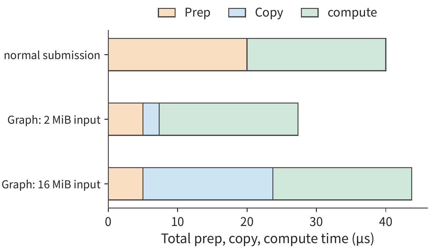
In Figure 5-33, the time graph replay saves in preparation is a fixed length, while the bar representing copy time grows longer as the input grows. When the two are equal, graph replay stops saving any time at all. Let the input data volume be X and the copy bandwidth be B; the condition for the graph to be faster is \(2X/B<15\ \mathrm{\mu s}\). Substituting B=1792 GB/s gives:

\[ X<\frac{15\times10^{-6}\times1.792\times10^{12}}{2}\ \mathrm{bytes}\approx12.8\ \mathrm{MiB}. \]

2 MiB is below this threshold, while 16 MiB exceeds it. Having the preceding operator write its result directly into the graph's buffer, or starting the capture from a point where the input tensor is smaller, can both reduce the copy overhead. So choosing which operations to combine into a graph requires weighing the saved host submission time against the added input-copy time.²²

Graph replay reuses the submission sequence; the same idea can also apply to the preparation work that precedes these tasks. For example, an execution plan can be shared across multiple model layers. The inference operator library FlashInfer separates plan generation (plan) from execution (run): plan selects kernels, partitions tasks, and arranges workspace based on this step's per-request lengths and where KV resides in GPU memory, and copies this metadata to the GPU; run then executes attention according to the plan. If, within the same step, all 36 layers have the same request lengths and the same KV layout, they can share a single plan; re-running plan for every layer would mean doing the same preparation work 36 times over. In two comparisons on the RTX PRO 6000, switching to a single plan call reduced the time for 36 layers of attention calls from about 2.0/2.4 ms to 0.72/0.75 ms, and reduced host-to-GPU copies from 144 to 4, while the number of accelerator kernels stayed the same. Conversely, once request lengths change, plan must be regenerated — reusing the old plan would compute against the old lengths and produce incorrect results.²³

5.5.3 Dynamic shape and compilation overhead

Multiple model layers sharing a plan relies on identical computation structure; different invocations sharing a compiled program must also handle changes in input shape. When the number of input rows changes, the runtime can choose among three approaches. A general-purpose program computes indices and bounds from the current shape; bucketing pads inputs to a small number of representative shapes and reuses the program for those shapes; specialization exploits known input conditions to generate a dedicated implementation — here, compiling a separate program for each common shape. The more fully known shapes are exploited, the more opportunity there is to simplify accelerator work, but this also requires compiling and storing more programs.

Example 5-12: How many repeated executions make specialization worthwhile? Take a group of 10 FFN calls: 8 with 256 rows, 1 with 1536 rows, and 1 with 2048 rows, totaling \(8\times256+1536+2048=5632\) rows. Using two buckets, 512 and 2048, the actual processed total is \(8\times512+2048+2048=8192\) rows, about 45% more computation. Figure 5-34 shows which bucket each actual row count is padded to.

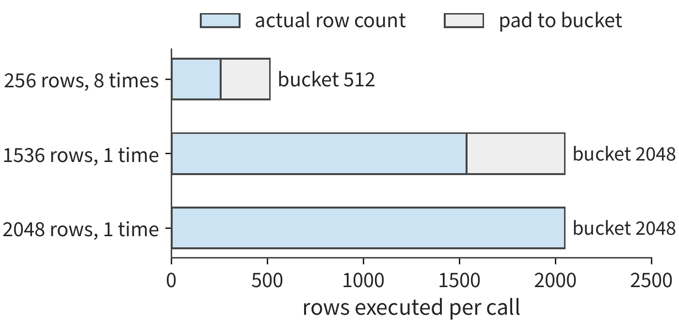
The three projections of a complete FFN require \(6HF\) FLOPs per row in total. On the RTX PRO 6000, taking the general-purpose, bucketed, and specialized implementations to reach about 20%, 40%, and 50% of the BF16 dense peak of 503.8 TFLOP/s — that is, MFU of 20%, 40%, and 50% — gives effective matrix processing rates of 100, 200, and 250 TFLOP/s, so each group takes roughly 17.0, 12.4, and 6.8 ms respectively. Although bucketing computes 45% more work, its processing rate doubles, so it is still faster than the general-purpose implementation. Suppose their preparation times are 100, 400, and 900 ms respectively; this gives the table below.²⁴

Strategy	One-time preparation P	Per-group execution T	Shape handling
General-purpose	100 ms	17.0 ms	Executes the actual 5632 rows
Bucketed	400 ms	12.4 ms	Padded to two buckets, executes 8192 rows
Per-shape specialized	900 ms	6.8 ms	Separate program generated for each of three shapes

The total time for running r groups is \(T_{\mathrm{total}}=P+rT\). In Figure 5-35, the intercept of each line represents the preparation time, and the slope represents the per-group execution time. In this example, the scheme that executes each group faster has a flatter line but a higher starting point, since it requires longer preparation.

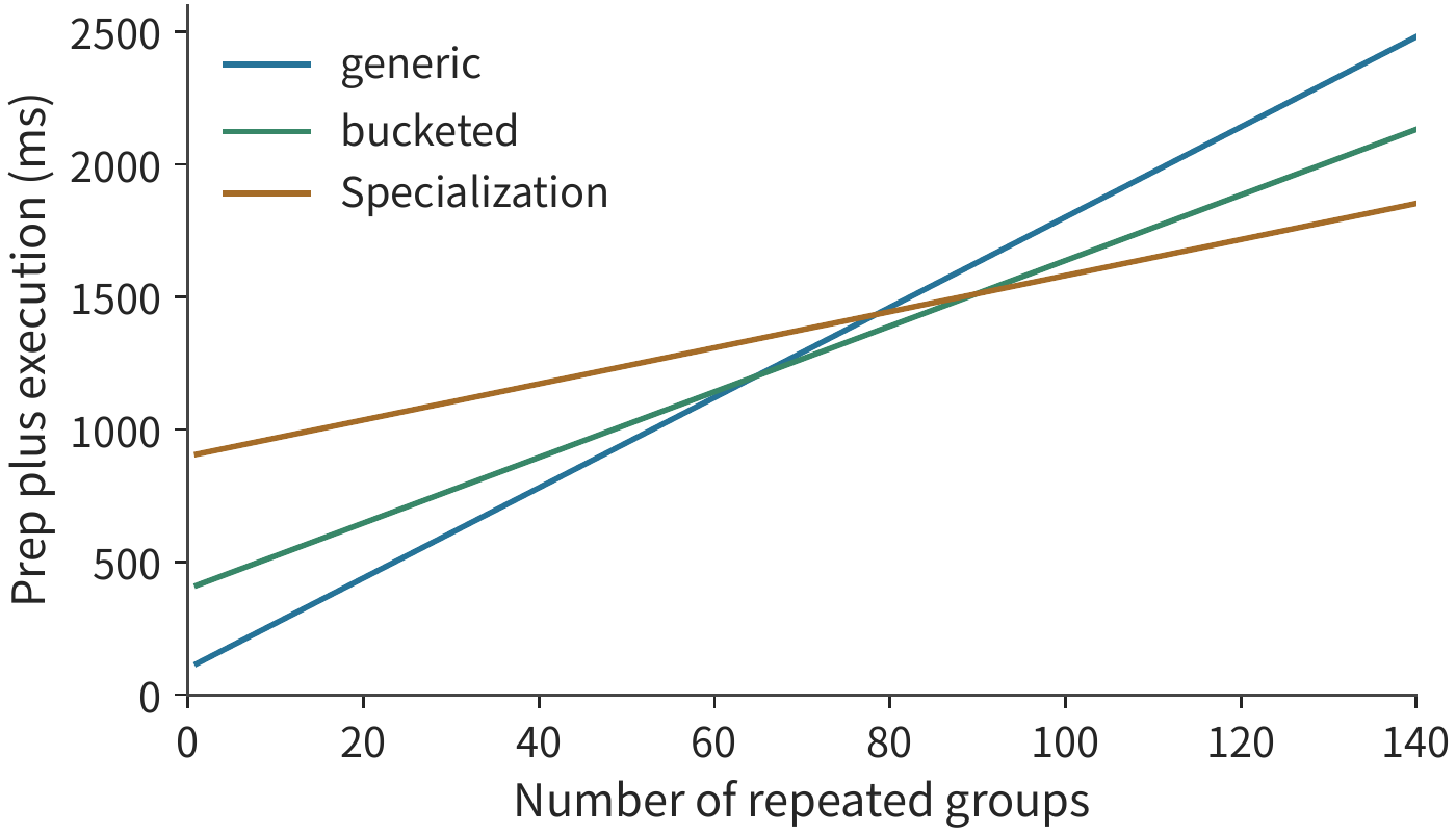
Bucketing uses 300 ms more preparation than the general-purpose scheme, but saves about 4.6 ms per group, so after about 65 groups the extra preparation is offset. Specialization uses another 500 ms more preparation than bucketing, saving about 5.6 ms more per group, requiring about 90 groups to offset. Computed from the exact values, general-purpose is cheapest for 1–64 groups, bucketed is cheapest for 65–89 groups, and specialization is cheapest from 90 groups onward.

If an instance runs only 70 groups, the total times are roughly 1.29, 1.27, and 1.38 s respectively. Bucketing takes the least time because its execution-time savings already exceed its extra preparation cost; although specialization executes each group faster, its cumulative time savings are not yet enough to offset the extra preparation overhead. If all three programs are already cached, the preparation cost for this run is zero, and specialization takes the least time starting from the first group. The runtime's choice therefore depends on both the frequency of each shape and whether the program has already been compiled and cached.

We can similarly compute how many calls are needed for auto-tuning to offset its preparation overhead. If a search takes 10 minutes and each call using the new implementation saves 5 μs, then offsetting the search time with cumulative savings requires \(600/(5\times10^{-6})=1.2\times10^8\) calls. At 10,000 calls per second, this takes about 3.3 hours; at 100 calls per second, about 14 days. The longer tuning takes, the more priority should go to optimizing shapes that are called frequently and used over a long period.

Chapter 8 will combine request arrival patterns with dynamic batching to further discuss how to select and cache programs. If a particular shape recurs repeatedly within a short time, keeping the corresponding compiled result reduces repeated preparation; if it is no longer used over the long term, that cache entry can be deleted to free space for other shapes.

5.5.4 Persistent kernel: scheduling tasks by data block

Graph replay and program caching reduce repeated host preparation, but there is another kind of waiting on the accelerator: for two kernels with a dependency, the latter usually still waits for the former to fully complete before starting. If the latter operator only needs one block of the former's result, the waiting condition can be narrowed to the data block: once the first block is ready, subsequent computation can begin immediately, while the remaining blocks continue computing.

A persistent kernel stays resident on the accelerator, pulling tasks from a queue and using events to confirm whether the required data is ready. This both reduces the host's repeated kernel-launch work and lets adjacent operators overlap execution by block. Mirage Persistent Kernel/MPK is a research system that adopts this task-scheduling approach.²⁶

Again using the up projection followed by SiLU activation in Qwen3-8B, take a feature vector of 512 tokens, grouped into eight blocks of 64 tokens each. Each block's projection is \(2\times64\times4096\times12288\approx6.44\) GFLOPs, taking about 12.8 μs at the RTX PRO 6000's BF16 dense peak of 503.8 TFLOP/s; each block's activation processes \(64\times12288\) BF16 elements, each reading 2 bytes and writing 2 bytes, taking about 1.76 μs at the memory bandwidth of 1792 GB/s. Assuming the matrix and vector resources are independent with ample buffering, and each kernel launch takes 5 μs, waiting for all projections to finish before starting activation takes a total of \(2\times5+8\times(12.8+1.76)\approx126\) μs.

Now split the computation into eight projection tasks and eight activation tasks, with each task adding 0.5 μs of scheduling time and 0.2 μs of completion-notification time. Each block's projection becomes 13.5 μs, and activation becomes 2.46 μs. With one kernel launch, the eight projection blocks run back-to-back, each block's activation starts immediately after its projection completes, and the last activation finishes after all projections are done, giving a completion time of \(5+8\times13.5+2.46\approx115\) μs, a speedup of about 1.1.

Here, the slower stage is projection. The roughly 11.0 μs saved comes from two sources: one fewer 5 μs kernel launch, and about 12.3 μs of the seven activation blocks hidden within the projection time; meanwhile, task overhead adds back 6.3 μs on the critical path. Since each activation block only takes 1.76 μs, starting it early per block can hide at most that much time. The closer the durations of the two stages, the more time block-wise overlap saves; when one stage is much longer than the other, the benefit is essentially limited to one fewer kernel launch.

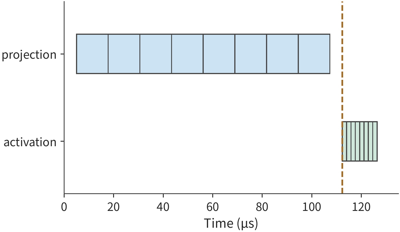
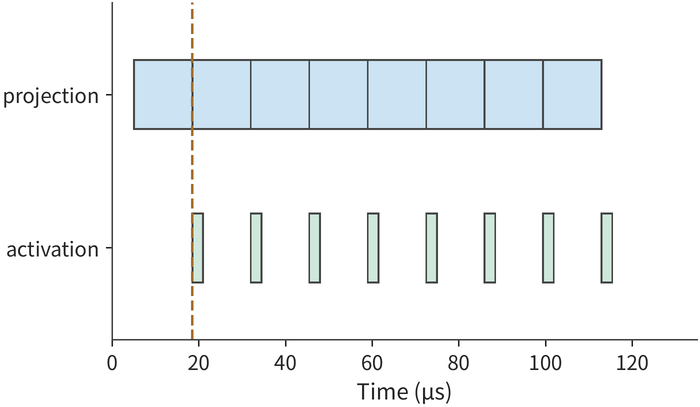
Following the projection timeline in Figure 5-37, the eight projection blocks run back-to-back with no gaps between them. This follows the same pattern as double buffering: the first block finishes the previous stage, and thereafter one block finishes every interval equal to the time needed by the slower stage — here, projection is the slower stage, just as movement was the slower stage in Section 5.3.2, and the pipeline's cadence is set by it. Each buffer slot stays occupied from the start of projection to the end of activation; when there is no free slot, the projection task must wait. The task queue, completion events, and free buffers thus jointly determine when the next block can start.

5.6 From local optimization to complete requests

Each optimization above has had a clearly defined target: tiling reduces repeated input reads, fusion reduces intermediate reads and writes, and runtime optimizations reduce preparation and waiting. But a complete request also includes other work, and the time saved locally is only a fraction of the total. This section first explains how to project request time from local speedups, then analyzes an actual request for Qwen3-8B.

5.6.1 Hotspot fraction determines the room for acceleration

Suppose a request consists of serial stages, the other stages' time stays unchanged, the hotspot accounts for a fraction f of the original time, and the hotspot's speedup is s. Normalizing the original request time to 1, the new time is \((1-f)+f/s\), and the overall speedup is:

\[ S_{\mathrm{request}}=\frac{1}{(1-f)+f/s}. \]

If the hotspot accounts for 20% and its speed doubles, the total time becomes \(0.8+0.2/2=0.9\), a speedup of about 1.11. Continuing to speed up the hotspot tenfold gives a total time of 0.82; even if the hotspot's time drops to zero, the other stages still take 0.8 of the original total time, so the overall speedup is capped at 1.25×.

This is Amdahl's law, introduced in Chapter 1. The law explains why optimization gains gradually shrink: the shorter the hotspot takes, the larger the fraction the other stages occupy in the total time.

5.6.2 Parallel branches and critical-path switching

In the Amdahl relationship, times add up along serial stages. If a request has two branches executing simultaneously, shortening one branch may still leave it waiting on the other; in that case, one should trace the dependency graph to find the longest path that determines the completion time. Suppose after 10 μs of preparation, hotspot A and branch B start simultaneously, taking 60 and 40 μs respectively; wrap-up takes 10 μs and waits for both branches to finish. The original request time is:

\[ T=10+\max(60,40)+10=80\ \mathrm{\mu s}. \]

Speeding up A fourfold to 15 μs, with B still taking 40 μs, gives a new time of \(10+\max(15,40)+10=60\) μs. A saves 45 μs, yet the request only saves 20 μs, because B replaces A as the critical path.

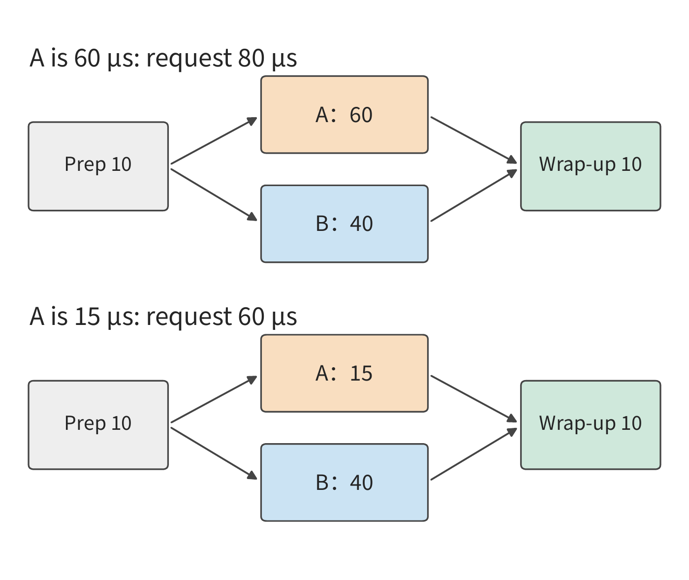
When A shrinks to 40 μs, it finishes exactly at the same time as B; continuing to optimize only A leaves the completion time stuck at 60 μs. This crossover point marks the maximum benefit obtainable from optimizing A alone. To shorten the request further, one should optimize B, or reduce preparation and wrap-up.

Shared resources can also change the branches' own times. Suppose A's new implementation heavily consumes bandwidth, causing the concurrently running B to take 90 μs instead; the request then becomes \(10+\max(15,90)+10=110\) μs. The extra time B takes exceeds the computation time A saved, and the whole request ends up slower instead.²⁷

The critical path shows that the time saved by one branch must be put back into the whole dependency graph to know how much faster the request actually becomes. Savings in storage must be put back into the whole execution process in the same way: a reduction in how much capacity a piece of state occupies is not necessarily equal to a reduction in bytes read per step, because how much is read per step depends on how many layers read it and which entries each layer reads. Section 2.3.6's V4.1 session already gave a set of numbers under an 8K condition: V4.1 has 38 global attention layers share 4 copies of global KV, cutting residency to about a quarter of V4-Flash's, yet the per-layer logical read only drops by about 9%, and that drop is smaller than the reduction in residency. Sharing state does not require each layer to store its own separate copy, but every layer that uses it still has to read it, so a reduction in capacity does not translate directly into a reduction in reads.³¹

As context grows longer, the index scan that still must run also brings more overhead. At 128K, the two generations' global historical state and logical index read volumes are about 65.085 and 33.422 MiB respectively. In V4.1, subsequent layers' index access only reaches the candidate pool, while the initial index still has to traverse the whole global state. So even though later layers' index access range is fixed, the overhead for the whole decode step still grows with context length.

What changes the cost is not only where the data comes from, but also whether the program truly avoids the computation. The candidate pool narrows the search range for later indices, reducing the workload accordingly. The public reference implementation first computes the dot product over the full cached index, then masks out positions outside the candidate pool; the paper's production implementation directly shrinks the number of entries scanned by later indices. The former has already performed the dot product outside the pool, while the latter skips that work at the point the computation is issued. The same selection rule thus corresponds to two different execution costs.

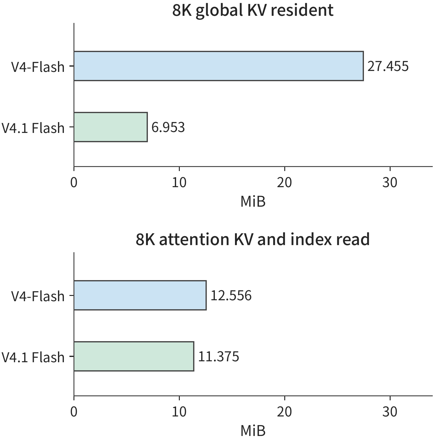
5.6.3 Comprehensive case: optimization choices for a Qwen3 request

Apply this method to Qwen3-8B on the RTX PRO 6000. The request input is 7239 tokens, generating 32 output tokens, with concurrency of 1, using BF16 and eager execution; here, eager means the host submits accelerator work item by item in program order. The model has 36 layers, first performing one prefill pass to produce the first output, then 31 decode passes. Each layer performs one SwiGLU activation per step, i.e., Section 5.3.1's \(Z=\operatorname{SiLU}(G)\odot U\), giving \(36\times32=1152\) calls in total, of which 36 are prefill and 1116 are decode.

The two kinds of calls carry different amounts of work. Within the same request, prefill executes this operator on 7239 input tokens across each of 36 model layers, processing \(36\times7239=260604\) token representations in total; the 31 decode steps each process one new token per layer, executing \(36\times31=1116\) single-token operator calls in total. Here we tally operator work as "number of layers × number of tokens," so the same token participating in multiple layers is counted repeatedly. Decode has 31 times as many calls as prefill, yet processes far fewer rows. This is exactly the shape difference this chapter has repeatedly encountered: large matrices offer more parallel work, small matrices take less compute time, and kernel-launch and task-dispatch overheads become more prominent and harder to hide, making it harder to fully utilize the accelerator.

Within the same engine, replacing the SwiGLU across all 36 layers with a kernel using a different scheduling scheme, and confirming from execution traces that all 1152 calls used the replacement kernel, gives the following stage timings.²⁸

SwiGLU stage	Call shape and count	Original kernel	Replacement kernel
Prefill	7239 rows, 36 calls	~11.2 ms	~11.2 ms
Decode	1 row, 1116 calls	~2.4 ms	~0.92 ms

The replacement kernel mainly shortens the decode activation time for single-row input, a speedup of about 2.6×, saving about 1.45 ms in total for the decode portion. The prefill activation time is essentially unchanged, actually taking about 0.03 ms more after the replacement. These activations execute serially with other accelerator work in the trace. The original kernel's total activation compute is about 13.6 ms, about 1.6% of the roughly 851 ms capture window; holding all other work fixed, even eliminating all activation compute would save at most 13.6 ms. Only the decode portion has been shortened so far, bringing total activation compute from 13.6 ms down to 12.2 ms, so the whole request is expected to drop by about 1.4 ms.

Measuring interleaved requests before and after the replacement on the client side gives 11 paired results. The first-token time before and after the replacement is about 436 ms in both cases, and the median complete-request time is about 817 ms and 815 ms respectively. Computing "time before replacement minus time after replacement" for each round, the median of the paired differences is about 1.3 ms, about 0.16% of the original request time, matching the expected ~1.4 ms. Figure 5-40 lists the difference for each round, with 9 pairs showing shorter time after the replacement and 2 pairs showing longer time.

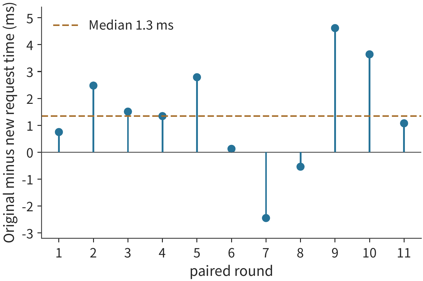
The decode improvement occurs after the first output, so for the current long-input request, the first-token time is still determined by the computation and waiting within prefill. The longer the output, the more times the single-row activation compute repeats, and the more the per-step savings accumulate.

When analyzing a complete request, first tally the call counts for each shape, then compute the time saved per call, and finally use the dependency structure to judge whether these savings shorten the whole request. This connects a kernel's speedup, the time each stage takes, and the time the user actually waits.

Common pitfalls

Pitfall: judging execution cost solely by kernel count. Graph replay reduced the host submissions for 3 FFN calls from 18 to 3, while the accelerator still executed 18 kernels; only fusion reduced the accelerator kernel count to 15. Host submission and accelerator computation should be interpreted along their own separate timelines.

Pitfall: the implementation with the smallest access volume is always fastest. Shrinking attention's K/V block from 64 rows to 1 row reduces access volume by 144 MiB, yet the number of state updates increases by about 41×. Reads, state updates, and matrix processing rate together determine execution cost.

Pitfall: adding buffers always improves throughput. On one H100 SM, each block takes 1.29 μs to move and 0.28 μs to compute; two slots already keep the mover working continuously, finishing four blocks in 5.44 μs. A third slot cannot make the movement faster, nor can speeding up the computation; to shorten the time, one must reduce the bytes moved per block or increase the bandwidth.

Pitfall: steady-state execution being fastest means the total time is shortest. Running 70 groups of calls, bucketing takes about 1.27 s while per-shape specialization takes about 1.38 s. Specialization executes each group faster, but the time saved is not yet enough to offset the extra preparation overhead.

Exercises and companion experiments

The following questions progressively vary the conditions of this chapter's examples. First complete the derivation on paper, then use the companion code or execution traces to explain the differences; the experiment entries retain their original numbering, with configuration, procedure, and full records in the corresponding materials.

Experiment 5-1 · Extension: how matrix block size changes local storage and read volume

Change Example 5-3's output block to 64×128, keeping the reduction block at 32, and find the local storage requirement, the read counts for A and W separately, and the total access volume. Compared with the 64×64 scheme, how much higher must the effective bandwidth of the 64×128 scheme be for its memory-access time to be shorter? Then compare execution traces for the two loop orders, and explain how contiguous access affects the processing rate.⁵

Experiment 5-2 · Core: how much memory access and GPU memory footprint can activation operator fusion reduce

For an activation chain with G and U each 24 MiB, draw the allocation, use, and release order of each tensor when the three operators execute independently versus when fully fused, and derive the 156 MiB and 60 MiB access volumes and the GPU memory footprint peaks for the two schemes. If the fused implementation adds a fixed 5 μs overhead per call, and the interface bandwidth is taken as the RTX PRO 6000's memory bandwidth of 1792 GB/s, how many input rows are needed at minimum for the memory-access time saved by fusion to exceed this overhead? Then, combining with the companion experiment results, explain the relationship between the reduction ratio in access volume and the reduction ratio in time.⁷

Experiment 5-3 · Extension: how blocked reduction and prefetching change attention computation and memory access

Add one more element to Example 5-6's input, with score \(\ln4\) and corresponding value 5, update m, \(\ell\), and u, and compare with processing three elements at once. Keeping the total attention buffer capacity at 99 KB (101,376 bytes), carve out an additional b×d BF16 prefetch slot, taking b=64, and find the new maximum number of Q rows, the number of scan passes, and the access volume. Explain why the prefetch buffer changes how many times data is read repeatedly.¹¹

Experiment 5-4 · Extension: does operator fusion change the computed result or the execution cost

In the pseudocode of Section 5.4.2, separately move SiLU inside the ko loop, remove the intermediate BF16 rounding, and move the quantization computation inside the loop over each output column block. State whether each change alters the mathematical operation, the numerical rounding, or the execution cost, and give an input that can distinguish the results or access volumes before and after each change.¹⁶

Experiment 5-5 · Extension: how blocked loops change access order and temporary storage

Write the i-k-j blocked loop using block indices and within-block coordinates, marking where the input cache and accumulator are created, last used, and released in the program. Then, against the companion transpose program's execution under two block sizes, compare access contiguity, synchronization operations, and temporary data volume, and use this to explain the difference in execution time.¹⁷

Experiment 5-6 · Extension: how the proportion of calls by input shape affects tuning benefit

Using Example 5-9's two input shapes, let shape A's call proportion be 1/2, 2/3, and 9/10 in turn, and compute the average time for the original and new implementations. If selecting the implementation by shape costs an extra 1 μs each time, using the new implementation for A and the original for B, when does this beat always using the original implementation? Then, based on the companion search records, tally the total search time, and compute how much execution time the found implementation saves across repeated calls.¹⁸

Experiment 5-7 · Extension: how many repeated executions does specialization need before it pays off

Draw the full timeline of preparation and execution in Example 5-12. Change the small shape's call count per group from 8 to 4, keeping the other two shapes at one call each. Compare each pair of schemes and find the repeat count at which their total times are equal. Then, assuming the two bucketed programs are already compiled and cached, find the repeat-count range over which each scheme has the shortest total time after the preparation times change.²⁴

Experiment 5-8 · Core: what overheads do graph replay and operator fusion each reduce

Read Figure 5-28 and tally the host submission count and accelerator kernel count for each of the four approaches. Move Example 5-11 to an RTX 4090, taking its copy bandwidth as its memory bandwidth of 1008 GB/s, and find the input data size at which the copy overhead exactly offsets the time saved by graph replay; then have the upstream operator write directly into the graph buffer, and compare the completion time of ordinary submission versus graph replay at input sizes of 2 MiB and 16 MiB.²⁵

Experiment 5-9 · Core: how kernel acceleration changes request time and the critical path

Using the companion 11 paired request records, first compute the time difference for each pair, then take the median of these differences. Explain how this differs from taking the median of each group of request times separately and then subtracting. Using the conditions of this chapter's comprehensive case, keep prefill unchanged and increase the number of decode steps from 31 to 127; assuming the per-step savings stay the same, estimate the total time savings in activation compute. Then progressively shorten A's execution time in Figure 5-38, and find the execution time of A at which the complete request time stops shortening further.²⁸

History and Further Reading

Halide separates algorithm from schedule, turning tiling, reordering, and compute placement into composable actions for the programmer; TVM connects tensor computation, backend generation, and automatic tuning; AKG combines polyhedral scheduling, hierarchical fusion, and on-chip storage arrangement for code generation on neural processors. Reading the original material behind all three lets you further trace how a given representation shapes which transformations a compiler can carry out automatically.¹⁴¹²

An FPGA is a configurable logic device; high-level synthesis (HLS) converts higher-level programs into hardware data paths. The author's early FPGA/HLS work also went through a shift from interface wrapping to code transformation: forming the required pipeline required identifying primitives and read/write dependencies, and changing the generated data path. This experience illustrates how the focus of the work shifted from simplifying programming to improving execution.

The operator orchestration optimization system Korch offers another instructive example: in one historical case, a subgraph originally executed as three kernels took about 91 μs in total; after being restructured into four kernels, the total dropped to about 69 μs. Re-splitting and recombining operators shortened accelerator execution time by enough to offset the extra kernel launch and data handoff overhead.¹³ Together with the fusion counterexample in this chapter, this direction shows that optimization should compare the cost of the entire computation process.

Chapter Summary

This chapter started from a single matrix projection and worked through memory access, operator fusion, compilation and runtime, ending with an analysis of the complete request. The sections repeatedly relied on three basic judgments.

First, reuse requires space. A larger output tile lets the same input participate in more multiply-adds, but it also requires more accumulator storage; keeping a quantized result around lets multiple column blocks read data at a lower bit width, but it also requires intermediate storage. Judging whether this storage is worthwhile means looking at how much rereading or recomputation it avoids. On an SM, this space also determines how many thread blocks can be resident, which in turn determines how many in-flight memory requests can hide latency.

Second, data dependencies determine computation order. An elementwise operation can complete as soon as the input at one position is ready, while a reduction must keep partial sums or online statistics. A compiler moves computation based on these dependencies, and a runtime uses events to confirm whether data is ready and whether a buffer can be released. Fusion and pipelining are both built on these dependency relationships.

Third, total time depends on the execution order of the various pieces of work. Bandwidth determines how long it takes to transfer a batch of data, the slower stage determines the completion interval between adjacent blocks in a pipeline, the number of reuses determines whether the resulting savings in execution time can offset the initial preparation time, and the critical path determines whether a local improvement can shorten the request. So it's necessary both to calculate how much work has been reduced and to determine whether that work actually affected the final completion time in the first place.

The next chapter extends these relationships to multiple accelerators. When a piece of result becomes ready, who needs to read it, and how long it must be kept will determine when communication can begin and how much buffering each end needs.

---

1. Fixed Qwen3-8B configuration; model operators and implementation. ↩

2. Tile capacity and data reuse, including loop counts, an Orojenesis excerpt, and bank mapping. ↩

3. Floating-point recomputation for split counts and merge order. This teaching row is generated from a given formula and then rounded to BF16; it is not a captured activation. Each square is exact in FP32, and the differences across paths come only from addition order. The exact value is computed with rationals and serves only as a comparison baseline; enumerating merge orders covers the possible sequences of atomic adds and does not represent the actual distribution on any particular backend. ↩

4. Three-stage split computation for RMSNorm. Input and gamma are BF16, with gamma read per row; one group retains the input for one row, and the three-stage scheme rereads the input at the application stage. ↩

5. Experiment 5-1, GPU tiling, reduction splitting. ↩↩

6. Fixed-scale fusion and tensor lifetime. ↩

7. Original conditions, data, and analysis for Experiment 5-2. RTX PRO 6000, shared GPU, warm cache, and graph replay; the original medians are 14.20/7.68 μs, measuring only the activation subchain. ↩↩

8. Streaming order and buffer budget; host transfer and buffer occupancy time. ↩↩

9. Attention tiling and online state; tile size and access volume under a 99 KB buffer. The capacity model assumes a single head, no masking, K/V reusing the input slots, and S/P reusing the temporary slots; the 99 KB shared-memory limit per thread block is taken from the CUDA Programming Guide's compute capability table (compute capability 12.x column). ↩

10. FlashAttention, FlashAttention-2, FlashAttention-3. ↩↩↩↩

11. Experiment 5-3. RTX PRO 6000 warm-cache single-head comparison: 2.64 ms/79.5 μs; the peak additional allocation was about 848/22.2 MiB, including the temporary amounts allocated by each backend. ↩↩

12. Zhao et al., 2021, AKG: Automatic Kernel Generation for Neural Processing Units using Polyhedral Transformations. ↩↩

13. Korch's orchestration case: in the paper's V100/FP32 subgraph, the three kernels take 38.7, 24.2, and 28.2 μs, and the four kernels take 7.6, 18.4, 7.5, and 35.7 μs. ↩

14. TVM, TensorIR. ↩↩

15. Fusion legality, FP8 rounding, and quantization projection; RedFuser backend reading. The 444/620 MiB counts include A, W, and the output; the auxiliary read/write for row scale is covered separately in the accompanying calculation. ↩↩

16. Compilation, rounding, and execution differences in Experiment 5-4, DeepSeek V4-Flash expert subchain. ↩↩

17. Generated code and transpose comparison for Experiment 5-5. ↩↩

18. Search and measurement records for Experiment 5-6; evaluation and deployment calculation. Two rounds totaling 12 agent calls were recorded, without producing a new, faster implementation. ↩↩

19. Host timeline research; configuration pipelining and graph execution. ↩

20. Archived vLLM v0.6.0 release announcement; for a discussion of attributing the benefit, see Section 8.2 of the token cost survey. The throughput in the announcement was measured with requests arriving simultaneously under --num-scheduler-steps 10; the 2.7x figure is the combined benefit of three changes and cannot be attributed entirely to the GIL. Multi-step scheduling can lengthen the wait for the first token under low load. ↩

21. Execution mode and feedback, framework evolution, and Sections 7–8 of the token cost survey. ↩

22. Small-input copying for graph replay, large-input copying, and graph execution trade-offs. Copy bandwidth is defined as the interface traffic of a source read plus a destination write. ↩

23. FlashInfer plan reuse measurement. ↩

24. Complete inputs and intersection points for shape specialization. ↩↩

25. Experiment 5-8 and trace analysis JSON. ↩↩

26. Device task organization and MPK; eight-block task computation. The projection is derived from the RTX PRO 6000's BF16 dense peak of 503.8 TFLOP/s, and the activation figure is derived from a 1792 GB/s memory bandwidth with 4 bytes read/write per element (448 G elements/s); both are taken from the hardware table. Independent resources, task overhead, and buffer conditions follow the settings used in the example. ↩

27. Teaching calculation for the request critical path, contention scenario. ↩

28. Kernel implementation, execution records, and 11 request pairs for Experiment 5-9. vLLM 0.23; the replacement kernel uses block256/4-warps scheduling, and the 11 output token pairs match. Client-side medians are 816.640/815.406 ms, the median of the paired time differences is 1.343 ms, and the first-token medians are 435.674/436.353 ms. In separately captured profiling records, prefill is 11.218659/11.244366 ms and decode is 2.369803/0.920376 ms. The original kernel took 13.588462 ms, the replacement took 12.164742 ms, and the capture window was 850.848989 ms; the intersection in time between each hotspot and other observed GPU work is zero. ↩↩

29. SM residency, latency hiding, and MMA instruction count, placing accumulators in registers, 1000 ns latency with 2 loads per warp. The SM limits are taken from the CUDA Programming Guide's compute capability table (compute capability 9.0 column) and the Hopper Tuning Guide; the definition of occupancy is taken from the Programming Guide's section on writing kernels; asynchronous copy, fences, warp division of labor, and swizzling are taken from the section on asynchronous data copies; the 3.35 TB/s figure is taken from the H100 product page; the 132 SMs and the BF16 dense matrix peak of 989.4 TFLOP/s are taken from the H100 Architecture Whitepaper (Table 3). Registers per thread, memory latency, outstanding loads per warp, load width, and the MMA instruction shape are values chosen for this section. ↩

30. CUDA execution model; synchronization semantics of the CUDA Runtime API; CUDA stream management and event management; PyTorch tutorial on pinned memory and asynchronous copies. Host copying and buffer reuse are also covered in the locally referenced calculation materials cited in this chapter. ↩↩

31. DeepSeek V4.1 official technical report, Sections 1, 2, 3, and 6; fixed conditions and recomputation for the cross-chapter thread. ↩

32. The RTX PRO 6000 Blackwell Workstation Edition specification lists the system interface as PCIe 5.0 x16; the NVIDIA H100 specification gives PCIe Gen5 x16 as 128 GB/s, which is the combined total for both directions, 64 GB/s per direction. ↩

33. The RTX PRO 6000 Blackwell is an SM120 architecture (see the execution environment for Experiment 5-2), i.e., compute capability 12.0; the CUDA Programming Guide's compute capability table gives, for that column, a shared-memory limit of 100 KB per SM and a limit of 99 KB per thread block, with the difference between the two being the 1 KiB reserved per block. ↩